Digital Modulations using Python 56-60페이지 참조
통신에서 활동되는 많은 변조 방식 가운데 하나인 BPSK 변조는 time domain 상에서 지속 시간이 Tb인 디지털 비트 데이터 "0"과 "1" 로 이루어진 신호를 각각 위상이 180도 차이가 나는 코사인 파형으로 변조하는 기법이다.
s1(t) = Ac cos(2π fct), 0 ≤ t ≤ Tb for binary 1
s0(t) = Ac cos(2π fct +π), 0 ≤ t ≤ Tb for binary 0
여기서 fc 는 변조 주파수를 뜻한다.
이러한 BPSK 변조파는 constellation diagram 상에서 실수축상에서 대칭을 이루는 두개의 점으로 표현이 가능하다.
BPSK 변조의 송신 transmitter 부분은 다음과 같이 구성된다. 변조된 신호는 (광)전송라인을 통해 보내지고 Coherent Receiver 에서 수신하게 된다. 이과정에서 노이즈를 탈 수 있으며 대표적인 노이즈가 바로 AWGN(Additive White Gaussian Noise) 이다. 이 노이즈는 변조도니 파형에 곱셈으로 작용하는 것이 아닌 덧셈 개념의 노이즈다. 즉 변조파형에 Gaussian 형태로 랜덤하게 가산되어 삐죽삐죽한 형상을 보여주게 되며 이과정에서 전송한 정보가 "0"인지 "1"인지 에러가 발생하게 되면 이 비율을 Bit Error Rate 약어로 BER이라고 한다. 이 부분은 다소 수학적이므로 별도로 언급할 예정이다.(참조:
BPSK변조에서 AGWN(Eb/No)노이즈에 의한 BER 이론 계산
https://blog.daum.net/ejleep1/1248 )

이러한 BPSK 변조과정을 전송되어 수신기에서 복조(Demodulation) 과정이 일어난다. BPSK 변조과정을 거친 데이터는 Coherent Receiver 를 사용하여 수신 후 복조가 가능하다. Coherent 라 함은 전송되는 변조 데이터의 주파수와 위상이 동일해야 함이 요구된다. 즉 변조 주파수와 위상을 정확히 알면 편하게 복조할 수 있다는 것이다. 실제로 전송 후 수신과정에서 알고 있는 전송주파수와 위상값 처리는 Costas loop 또는 PLL(Phase Locked Koop) 가 담당하게 된다. 아래 그림에서 Costas loop 로 처리돈 부분이 rbb(t) 라 보면 될 것이다.
복조과정에서 rbb(t) 는 전송과정에서 노이즈를 타기때문에 원래의 파형 형상을 유지하지는 못할 것이다. 따라서 전송된 NRZ 코드 즉 "+1"인지 아니면 "-1"인지를 판단하는 기준은 즉 threshold 값으로서 "0"V 가 될 것이다. 왜 BPSK 변조 과정에서 "0"V 사용을 배제하는 주된 이유가 바로 그것이다. rbb(t) 값을 1비트 지속시간 동안 적분하고 그 결과치가 "0" 이상인지 아닌지를 확인하여 신호를 복조하여 내는 것이다. 이와같이 복조헤서 얻어지는 신호에 "^" 기호로 처리 후 이론적인 BER 계산에 사용하기로 하자. "^" 기호로 처리된 이 부분은 실제 통신에서 사용하는 양이므로 하드웨어 및 소프트웨어에서 원 신호와 차이가 최소화 될 수 있도록 처리되어야 하며 일명 "optimal"값 이라 한다. 물론 여러가지 방법이 있을 수 있다.
이러한 "0"과 "1" 로만 이루어진 신호를 코사인 변조주파수를 사용한 코사인 변조 파형 및 constellation diagram 을 matplotlib 라이브러리를 사용하여 작도해보자. 아울러 변조파형에 AWGN(additive white Gaussian Noise) 를 추가해 보자. AWGN 은 -4dB에서 2 dB 씩 증분하여 7가지 경우를 계산하여 중첩 작도하였다. 노이즈를 탄 개별 파형을 보려면 for loop 부분을 수정해야 할 것이다.
한편 Bit Error 계산 결과 작도는 앞으로 별도로 해설을 올릴 예정이다.(참조: BPSK변조에서 AGWN(Eb/No)노이즈에 의한 BER 이론 계산https://blog.daum.net/ejleep1/1248 )
BPSK_MODIFIED.PY의 코드 시작 부분을 살펴 보기로 한다.
첫번째 비트 신호 생성에 관해서 살펴 보자.
전송해야 할 심볼의 수를 100000개로 설정하자. 심볼의 종류는 위 그래프 상에서 constellation diagram의 점 또는 점 주위에 모인 군집으로 나타낼 수 있으며 BPSK에서는 2개로 볼 수 있다. 아울러 "1" 또는 "0" 각각이 하나의 심볼이며 이들은 전송전에 NRZ(non return zero)코딩에 의해 예를 들면 "+1V" 와 "-1" 로 처리하여 좌표 평면 상에서 y 축에 대칭인 점들로 constellation diagram 상에 위치하게 된다.
N 값은 충분히 큰 수값을 취하게 되는데 carrier 의 주파수나 또는 sampling 주파수에 의해 요구되는 최소한의 Nykist criteria 보다 더 클 필요가 있다. 즉 sampling 주파수의 2배 이상으로 큰 값이 좋다. 으며 시간적으로 말하자면 배수* 초당sampling 주파수에 해당하는 심볼수를 가지게 된다.
carrier 주파수가 800Hz 이고 oversampling rate 이 16 이면 sampling 주파수가 12800 Hz 가 된다. 따라서 N=100000이면 거의 7.8초 가량이므로 충분하다고 볼 수 있다.
N=100000 # Number of symbols to transmit
ENN0dB는 Eb/N0 비율을 일반적으로 start= -4dB에서 stop = -2, 0, 2, 4, 6, 8, 10dB 로 두고 step = 2dB 로 둔다.
EbN0dB = np.arange(start=10,stop = 10.5,step = 2) # Eb/N0 range in dB for simulation
L 은 oversampling factor로 10 이상의 충분히 큰 수로 잡자.
L=16 # oversampling factor,L=Tb/Ts(Tb=bit period,Ts=sampling period)
# if a carrier is used, use L = Fs/Fc, where Fs >> 2xFc
Fc=800 # carrier frequency
Fs=L*Fc # sampling frequency
BER 값을 0.0으로 초기화 한다.
BER = np.zeros(len(EbN0dB)) # for BER values for each Eb/N0
radint(2, size=N)은 0과 같거나 큰 2보다는 작은 정수형 난수를 N개 만큼 생성하여 array ak 를 준비한다.
ak = np.random.randint(2, size=N) # uniform random symbols from 0's and 1's
channels.py 코드에 포함된 bpsk_mod(ak,L) 함수를 사용하여 NRZ baseband 코드인 s_bb 를 생성한다.
그 갯수는 N개만큼 생성된 ak 의 L배 만큼이다. 이는 t의 np.arrange 명령에 의한 시간간격 생성에서 시작이 0 이고 마지막이 len(ak)*L이라는 사실에서 알 수 있다.
(s_bb,t)= bpsk_mod(ak,L) # BPSK modulation(waveform) - baseband
코사인 파형의 캐리어 파형을 생성하여 s_bb 로 변조한다.
s = s_bb*np.cos(2*np.pi*Fc*t/Fs) # with carrier
생성된 변조 파형이 위 그림의 2번째 파형이다. 이 파형의 주파수 특성을 관찰하기 위한 DFT 처리는 다음 url 을 방문하여 참고하기 바란다. (DFT 신호처리 및 AWGN효과 시각화: https://blog.daum.net/ejleep1/1252)
BPSK 시뮬레이션을 통해 마치 baseband 신호 ak 가 전송중에 white 노이즈를 탄 것처럼 조작 후 다시 복조하고 원 baseband 신호와 차이가 있는지 체크하여 평균을 구하여 시뮬레이션 BER 값으로 둔다.
한편 ak는 0.0과 1.0 으로 표현되는 리스트 데이터인 반면에 ak_hat는 Boolean 으로 표현된다. 이들이 일치하지 않으면 1만큼씩 카운트 합산된다. ( 이 숫자 "0.0"과 "1.0" 인 데이터와 "False"와 "True" 인 데이터를 비교해서 처리하는 이 파이선 명령 사용법은 실제 예제를 만들어 실행해 보아야 이해가 된다.)
Eb/N0dB 값에 따른 복조(demodulation) 과정을 살펴보자. 전송 준비된 신호 s에 white noise 를 부가할 수 있도록 channels.py 에 포함되어 있는 함수 awgn 을 사용하자. 이렇게 처리된 신호 데이터를 함수 bpsk_demod() 를 사용하여 복조(demodulation) 하도록 하자.
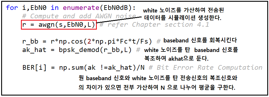
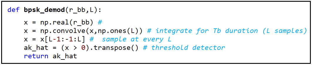
복조를 위한 코드를 살펴보면 전송하고자 하는 심볼 수인 N개에 해당하는 만큼 생성된 "_1"과 "+1" 이루어진 데이터를 처리함에 있어서 변조에서와 마찬가지로 N개의 데이터 r_bb 와 L 즉 oversampling rate 이 필요하다.
np.ones(L) 의 실행은 L개의 원소를 갖는 리스트 데이터 즉 [1., 1., 1., 1., ..., 1.]가 생성된다.
디폴트 조건의 convolve 명령은 컨볼루션 적분을 수행한다. 현재 np.ones(L)을 커늘로 하여 1차원적으로 리스트 데이터 x 를 +1씩 스트라이딩하며 결과를 생성한다. 하지만 첫 컨볼루션에서 (L-1)개 만큼은 padding x 데이터가 없으므로 0 으로 처리하면 L번째와 x의 첫번째 데이터와의 곱만이 남는다. 이런 방식으로 1씩 스트라이딩 하면서 L 개의 컨볼루션 값을 구해서 합산하도록 하는데 이것이 바로 적분을 뜻하는 듯 하다. (현재 간격 사이를 1 로 보기때문에 L 값으로 나누어야 정확한 적분 값이 되지 않을까 한다.) 하지만 이어지는 계산에서 결과가 단지 0보다 큰지 작은지만을 체크하기 때문에 문제가 될 것은 없다.
x[L-1:-1:L]에서 첫법째 인덱스 L-1 은 앞서 거론했던 padding 없는 부분까지의 갯수를 감안허여 적어도 x의 첫번째 데이터가 사용되는 지점까지를 의미하는데 x 로서는 첫번째 0에 해당하는 위치이며 :-1 은 x의 L-1 번째 데이터를 지정한다. 마지막의 :L은 L개 단위로 건너 뛰면서 적분 값을 계산한다는 의미이다.
마지막 (x>0).transpose( ) 명령에서 .transpose( ) 는 별 의미가 없어 보인다. 이 명령 없이 추력해도 결과는 마찬가지로 확인되었다.
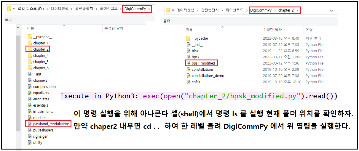
첨부된 파이선 코드를 실행해보자. 아나콘다에서 실행을 위해서 아래의 bpsk_modified.py를 실행하자.
폴더 구조를 살펴보면 현재 chapter_2 내부에 이 코드가 포함되어 있다.
아울러 passband_modulations.py 도 같은 chapter_2 폴더와 함께 위치하고 있어야 bpsk_modified.py 가 불러서 사용하게 된다. 코드 bpsk_modified 는 원래 subplot 명령을 사용하여 아주 작은 크기로 출력되기때문에 큼직한 그래프를 출력하도록 변경하였다.
물론 이 코드에는 BPSK 이외도 많은 변조 방식 시뮬레이션을 지원하는 코드들이 들어 있으므로 앞으로 다른 변조방식에 대한 블로그 작성 시 지속적으로 사용할 예정이다. 따라서 셸(shell)에서 cd .. 명령을 사용하여 chapter_2로부터 DigicommPy 로 변경 후 exec(open("chapter_2/bpsk_modified.py").read()) 명령을 실행하자.
아래 그림의 폴더 구조를 참조 확인하여 실행하도록 하자.
코드 실행하는 요령을 다음 보기 YouTube 를 클릭하여 살펴보세요. 구독 좋아요 부탁해요!
Under Construction ...
#BPSK_modified.py
#Execute in Python3: exec(open("chapter_2/bpsk_modified.py").read())
import numpy as np #for numerical computing
import matplotlib.pyplot as plt #for plotting functions
from passband_modulations import bpsk_mod, bpsk_demod
from channels import awgn
from scipy.special import erfc
N=100000 # Number of symbols to transmit
print(N)
EbN0dB = np.arange(start=-4,stop = 11,step = 2) # Eb/N0 range in dB for simulation
L=16 # oversampling factor,L=Tb/Ts(Tb=bit period,Ts=sampling period)
# if a carrier is used, use L = Fs/Fc, where Fs >> 2xFc
Fc=800 # carrier frequency
Fs=L*Fc # sampling frequency
BER = np.zeros(len(EbN0dB)) # for BER values for each Eb/N0
ak = np.random.randint(2, size=N) # uniform random symbols from 0's and 1's
(s_bb,t)= bpsk_mod(ak,L) # BPSK modulation(waveform) - baseband
s = s_bb*np.cos(2*np.pi*Fc*t/Fs) # with carrier
# Waveforms at the transmitter
fig1 = plt.figure(figsize=(10,5))
plt.plot(t,s_bb) # baseband wfm zoomed to first 10 bits
plt.xlabel('t(s)');plt.ylabel(r'$s_{bb}(t)$-baseband')
plt.xlim(0,10*L)
plt.show()
fig2 = plt.figure(figsize=(10,5))
plt.plot(t,s) # transmitted wfm zoomed to first 10 bits
plt.xlabel('t(s)');plt.ylabel('s(t)-with carrier')
plt.xlim(0,10*L)
plt.show()
#signal constellation at transmitter
fig3 = plt.figure(figsize=(5,5))
plt.plot(np.real(s_bb),np.imag(s_bb),'o')
plt.xlim(-1.5,1.5)
plt.ylim(-1.5,1.5)
plt.show()
fig4 = plt.figure(figsize=(10,5))
for i,EbN0 in enumerate(EbN0dB):
# Compute and add AWGN noise
r = awgn(s,EbN0,L) # refer Chapter section 4.1
r_bb = r*np.cos(2*np.pi*Fc*t/Fs) # recovered baseband signal
ak_hat = bpsk_demod(r_bb,L) # baseband correlation demodulator
BER[i] = np.sum(ak !=ak_hat)/N # Bit Error Rate Computation
# Received signal waveform zoomed to first 10 bits
plt.plot(t,r) # received signal (with noise)
plt.xlabel('t(s)');plt.ylabel('r(t)')
plt.xlim(0,10*L)
plt.show()
#------Theoretical Bit/Symbol Error Rates-------------
theoreticalBER = 0.5*erfc(np.sqrt(10**(EbN0dB/10))) # Theoretical bit error rate
#-------------Plots---------------------------
fig5, ax1 = plt.subplots(nrows=1,ncols = 1)
ax1.semilogy(EbN0dB,BER,'k*',label='Simulated') # simulated BER
ax1.semilogy(EbN0dB,theoreticalBER,'r-',label='Theoretical')
ax1.set_xlabel(r'$E_b/N_0$ (dB)')
ax1.set_ylabel(r'Probability of Bit Error - $P_b$')
ax1.set_title(['Probability of Bit Error for BPSK modulation'])
ax1.legend();plt.show()
#pasband_moulations.py
"""
Passband simulation models - modulation and demodulation techniques (Chapter 2)
@author: Mathuranathan Viswanathan
Created on Jul 17, 2019
"""
import numpy as np
import matplotlib.pyplot as plt
def bpsk_mod(ak,L):
"""
Function to modulate an incoming binary stream using BPSK (baseband)
Parameters:
ak : input binary data stream (0's and 1's) to modulate
L : oversampling factor (Tb/Ts)
Returns:
(s_bb,t) : tuple of following variables
s_bb: BPSK modulated signal(baseband) - s_bb(t)
t : generated time base for the modulated signal
"""
from scipy.signal import upfirdn
s_bb = upfirdn(h=[1]*L, x=2*ak-1, up = L) # NRZ encoder
t=np.arange(start = 0,stop = len(ak)*L) #discrete time base
return (s_bb,t)
def bpsk_demod(r_bb,L):
"""
Function to demodulate a BPSK (baseband) signal
Parameters:
r_bb : received signal at the receiver front end (baseband)
L : oversampling factor (Tsym/Ts)
Returns:
ak_hat : detected/estimated binary stream
"""
x = np.real(r_bb) # I arm
x = np.convolve(x,np.ones(L)) # integrate for Tb duration (L samples)
x = x[L-1:-1:L] # I arm - sample at every L
ak_hat = (x > 0).transpose() # threshold detector
return ak_hat
def add_awgn_noise(s,SNRdB,L=1):
"""
Function to add AWGN noise to input signal
The function adds AWGN noise vector to signal 's' to generate a \
resulting signal vector 'r' of specified SNR in dB. It also returns\
the noise vector 'n' that is added to the signal 's' and the spectral\
density N0 of noise added
Parameters:
s : input/transmitted signal vector
SNRdB : desired signal to noise ratio (expressed in dB)
for the received signal
L : oversampling factor (applicable for waveform simulation)
default L = 1.
Returns:
(r,n,N0) : tuple of following variables
r : received signal vector (r = s+n)
n : noise signal vector added
N0 : spectral density of the generated noise vector n
"""
gamma = 10**(SNRdB/10) #SNR to linear scale
if s.ndim==1:# if s is single dimensional vector
P=L*np.sum(abs(s)**2)/len(s) #Actual power in the vector
else: # multi-dimensional signals like MFSK
P=L*np.sum(np.sum(abs(s)**2))/len(s) # if s is a matrix [MxN]
N0=P/gamma # Find the noise spectral density
from numpy.random import standard_normal
if np.isrealobj(s):# check if input is real/complex object type
n = np.sqrt(N0/2)*standard_normal(s.shape) # computed noise
else:
n = np.sqrt(N0/2)*(standard_normal(s.shape)+1j*standard_normal(s.shape)) #computed noise
r = s + n # received signal
return (r,n,N0)
def qpsk_mod(a, fc, OF, enable_plot = False):
"""
Modulate an incoming binary stream using conventional QPSK
Parameters:
a : input binary data stream (0's and 1's) to modulate
fc : carrier frequency in Hertz
OF : oversampling factor - at least 4 is better
enable_plot : True = plot transmitter waveforms (default False)
Returns:
result : Dictionary containing the following keyword entries:
s(t) : QPSK modulated signal vector with carrier i.e, s(t)
I(t) : baseband I channel waveform (no carrier)
Q(t) : baseband Q channel waveform (no carrier)
t : time base for the carrier modulated signal
"""
L = 2*OF # samples in each symbol (QPSK has 2 bits in each symbol)
I = a[0::2];Q = a[1::2] #even and odd bit streams
# even/odd streams at 1/2Tb baud
from scipy.signal import upfirdn #NRZ encoder
I = upfirdn(h=[1]*L, x=2*I-1, up = L)
Q = upfirdn(h=[1]*L, x=2*Q-1, up = L)
fs = OF*fc # sampling frequency
t=np.arange(0,len(I)/fs,1/fs) #time base
I_t = I*np.cos(2*np.pi*fc*t);Q_t = -Q*np.sin(2*np.pi*fc*t)
s_t = I_t + Q_t # QPSK modulated baseband signal
if enable_plot:
fig = plt.figure(constrained_layout=True)
from matplotlib.gridspec import GridSpec
gs = GridSpec(3, 2, figure=fig)
ax1 = fig.add_subplot(gs[0, 0]);ax2 = fig.add_subplot(gs[0, 1])
ax3 = fig.add_subplot(gs[1, 0]);ax4 = fig.add_subplot(gs[1, 1])
ax5 = fig.add_subplot(gs[-1,:])
# show first few symbols of I(t), Q(t)
ax1.plot(t,I);ax1.set_title('I(t)')
ax2.plot(t,Q);ax2.set_title('Q(t)')
ax3.plot(t,I_t,'r');ax3.set_title('$I(t) cos(2 \pi f_c t)$')
ax4.plot(t,Q_t,'r');ax4.set_title('$Q(t) sin(2 \pi f_c t)$')
ax1.set_xlim(0,20*L/fs);ax2.set_xlim(0,20*L/fs)
ax3.set_xlim(0,20*L/fs);ax4.set_xlim(0,20*L/fs)
ax5.plot(t,s_t);ax5.set_xlim(0,20*L/fs);fig.show()
ax5.set_title('$s(t) = I(t) cos(2 \pi f_c t) - Q(t) sin(2 \pi f_c t)$')
result = dict()
result['s(t)'] =s_t;result['I(t)'] = I;result['Q(t)'] = Q;result['t'] = t
return result
def qpsk_demod(r,fc,OF,enable_plot=False):
"""
Demodulate a conventional QPSK signal
Parameters:
r : received signal at the receiver front end
fc : carrier frequency (Hz)
OF : oversampling factor (at least 4 is better)
enable_plot : True = plot receiver waveforms (default False)
Returns:
a_hat - detected binary stream
"""
fs = OF*fc # sampling frequency
L = 2*OF # number of samples in 2Tb duration
t=np.arange(0,len(r)/fs,1/fs) # time base
x=r*np.cos(2*np.pi*fc*t) # I arm
y=-r*np.sin(2*np.pi*fc*t) # Q arm
x = np.convolve(x,np.ones(L)) # integrate for L (Tsym=2*Tb) duration
y = np.convolve(y,np.ones(L)) #integrate for L (Tsym=2*Tb) duration
x = x[L-1::L] # I arm - sample at every symbol instant Tsym
y = y[L-1::L] # Q arm - sample at every symbol instant Tsym
a_hat = np.zeros(2*len(x))
a_hat[0::2] = (x>0) # even bits
a_hat[1::2] = (y>0) # odd bits
if enable_plot:
fig, axs = plt.subplots(1, 1)
axs.plot(x[0:200],y[0:200],'o');fig.show()
return a_hat
def oqpsk_mod(a,fc,OF,enable_plot=False):
"""
Modulate an incoming binary stream using OQPSK
Parameters:
a : input binary data stream (0's and 1's) to modulate
fc : carrier frequency in Hertz
OF : oversampling factor - at least 4 is better
enable_plot : True = plot transmitter waveforms (default False)
Returns:
result : Dictionary containing the following keyword entries:
s(t) : QPSK modulated signal vector with carrier i.e, s(t)
I(t) : baseband I channel waveform (no carrier)
Q(t) : baseband Q channel waveform (no carrier)
t : time base for the carrier modulated signal
"""
L = 2*OF # samples in each symbol (QPSK has 2 bits in each symbol)
I = a[0::2];Q = a[1::2] #even and odd bit streams
# even/odd streams at 1/2Tb baud
from scipy.signal import upfirdn #NRZ encoder
I = upfirdn(h=[1]*L, x=2*I-1, up = L)
Q = upfirdn(h=[1]*L, x=2*Q-1, up = L)
I = np.hstack((I,np.zeros(L//2))) # padding at end
Q = np.hstack((np.zeros(L//2),Q)) # padding at start
fs = OF*fc # sampling frequency
t=np.arange(0,len(I)/fs,1/fs) #time base
I_t = I*np.cos(2*np.pi*fc*t);Q_t = -Q*np.sin(2*np.pi*fc*t)
s = I_t + Q_t # QPSK modulated baseband signal
if enable_plot:
fig = plt.figure(constrained_layout=True)
from matplotlib.gridspec import GridSpec
gs = GridSpec(3, 2, figure=fig)
ax1 = fig.add_subplot(gs[0, 0]);ax2 = fig.add_subplot(gs[0, 1])
ax3 = fig.add_subplot(gs[1, 0]);ax4 = fig.add_subplot(gs[1, 1])
ax5 = fig.add_subplot(gs[-1,:])
# show first few symbols of I(t), Q(t)
ax1.plot(t,I);ax1.set_title('I(t)')
ax2.plot(t,Q);ax2.set_title('Q(t)')
ax3.plot(t,I_t,'r');ax3.set_title('$I(t) cos(2 \pi f_c t)$')
ax4.plot(t,Q_t,'r');ax4.set_title('$Q(t) sin(2 \pi f_c t)$')
ax1.set_xlim(0,20*L/fs);ax2.set_xlim(0,20*L/fs)
ax3.set_xlim(0,20*L/fs);ax4.set_xlim(0,20*L/fs)
ax5.plot(t,s);ax5.set_xlim(0,20*L/fs);fig.show()
ax5.set_title('$s(t) = I(t) cos(2 \pi f_c t) - Q(t) sin(2 \pi f_c t)$')
fig, axs = plt.subplots(1, 1)
axs.plot(I,Q);fig.show()#constellation plot
result = dict()
result['s(t)'] =s;result['I(t)'] = I;result['Q(t)'] = Q;result['t'] = t
return result
def oqpsk_demod(r,N,fc,OF,enable_plot=False):
"""
Demodulate a OQPSK signal
Parameters:
r : received signal at the receiver front end
N : Number of OQPSK symbols transmitted
fc : carrier frequency (Hz)
OF : oversampling factor (at least 4 is better)
enable_plot : True = plot receiver waveforms (default False)
Returns:
a_hat - detected binary stream
"""
fs = OF*fc # sampling frequency
L = 2*OF # number of samples in 2Tb duration
t=np.arange(0,(N+1)*OF/fs,1/fs) # time base
x=r*np.cos(2*np.pi*fc*t) # I arm
y=-r*np.sin(2*np.pi*fc*t) # Q arm
x = np.convolve(x,np.ones(L)) # integrate for L (Tsym=2*Tb) duration
y = np.convolve(y,np.ones(L)) #integrate for L (Tsym=2*Tb) duration
x = x[L-1:-1-L:L] # I arm - sample at every symbol instant Tsym
y = y[L+L//2-1:-1-L//2:L] # Q arm - sample at every symbol starting at L+L/2-1th sample
a_hat = np.zeros(N)
a_hat[0::2] = (x>0) # even bits
a_hat[1::2] = (y>0) # odd bits
if enable_plot:
fig, axs = plt.subplots(1, 1)
axs.plot(x[0:200],y[0:200],'o');fig.show()
return a_hat
def piBy4_dqpsk_Diff_encoding(a,enable_plot=False):
"""
Phase Mapper for pi/4-DQPSK modulation
Parameters:
a : input stream of binary bits
Returns:
(u,v): tuple, where
u : differentially coded I-channel bits
v : differentially coded Q-channel bits
"""
from numpy import pi, cos, sin
if len(a)%2: raise ValueError('Length of binary stream must be even')
I = a[0::2] # odd bit stream
Q = a[1::2] # even bit stream
# club 2-bits to form a symbol and use it as index for dTheta table
m = 2*I+Q
dTheta = np.array([-3*pi/4, 3*pi/4, -pi/4, pi/4]) #LUT for pi/4-DQPSK
u = np.zeros(len(m)+1);v = np.zeros(len(m)+1)
u[0]=1; v[0]=0 # initial conditions for uk and vk
for k in range(0,len(m)):
u[k+1] = u[k] * cos(dTheta[m[k]]) - v[k] * sin(dTheta[m[k]])
v[k+1] = u[k] * sin(dTheta[m[k]]) + v[k] * cos(dTheta[m[k]])
if enable_plot:#constellation plot
fig, axs = plt.subplots(1, 1)
axs.plot(u,v,'o');
axs.set_title('Constellation');fig.show()
return (u,v)
def piBy4_dqpsk_mod(a,fc,OF,enable_plot = False):
"""
Modulate a binary stream using pi/4 DQPSK
Parameters:
a : input binary data stream (0's and 1's) to modulate
fc : carrier frequency in Hertz
OF : oversampling factor
Returns:
result : Dictionary containing the following keyword entries:
s(t) : pi/4 QPSK modulated signal vector with carrier
U(t) : differentially coded I-channel waveform (no carrier)
V(t) : differentially coded Q-channel waveform (no carrier)
t: time base
"""
(u,v)=piBy4_dqpsk_Diff_encoding(a) # Differential Encoding for pi/4 QPSK
#Waveform formation (similar to conventional QPSK)
L = 2*OF # number of samples in each symbol (QPSK has 2 bits/symbol)
U = np.tile(u, (L,1)).flatten('F')# odd bit stream at 1/2Tb baud
V = np.tile(v, (L,1)).flatten('F')# even bit stream at 1/2Tb baud
fs = OF*fc # sampling frequency
t=np.arange(0, len(U)/fs,1/fs) #time base
U_t = U*np.cos(2*np.pi*fc*t)
V_t = -V*np.sin(2*np.pi*fc*t)
s_t = U_t + V_t
if enable_plot:
fig = plt.figure(constrained_layout=True)
from matplotlib.gridspec import GridSpec
gs = GridSpec(3, 2, figure=fig)
ax1 = fig.add_subplot(gs[0, 0]);ax2 = fig.add_subplot(gs[0, 1])
ax3 = fig.add_subplot(gs[1, 0]);ax4 = fig.add_subplot(gs[1, 1])
ax5 = fig.add_subplot(gs[-1,:])
ax1.plot(t,U);ax2.plot(t,V)
ax3.plot(t,U_t,'r');ax4.plot(t,V_t,'r')
ax5.plot(t,s_t) #QPSK waveform zoomed to first few symbols
ax1.set_ylabel('U(t)-baseband');ax2.set_ylabel('V(t)-baseband')
ax3.set_ylabel('U(t)-with carrier');ax4.set_ylabel('V(t)-with carrier')
ax5.set_ylabel('s(t)');ax5.set_xlim([0,10*L/fs])
ax1.set_xlim([0,10*L/fs]);ax2.set_xlim([0,10*L/fs])
ax3.set_xlim([0,10*L/fs]);ax4.set_xlim([0,10*L/fs])
fig.show()
result = dict()
result['s(t)'] =s_t;result['U(t)'] = U;result['V(t)'] = V;result['t'] = t
return result
def piBy4_dqpsk_Diff_decoding(w,z):
"""
Phase Mapper for pi/4-DQPSK modulation
Parameters:
w - differentially coded I-channel bits at the receiver
z - differentially coded Q-channel bits at the receiver
Returns:
a_hat - binary bit stream after differential decoding
"""
if len(w)!=len(z): raise ValueError('Length mismatch between w and z')
x = np.zeros(len(w)-1);y = np.zeros(len(w)-1);
for k in range(0,len(w)-1):
x[k] = w[k+1]*w[k] + z[k+1]*z[k]
y[k] = z[k+1]*w[k] - w[k+1]*z[k]
a_hat = np.zeros(2*len(x))
a_hat[0::2] = (x > 0) # odd bits
a_hat[1::2] = (y > 0) # even bits
return a_hat
def piBy4_dqpsk_demod(r,fc,OF,enable_plot=False):
"""
Differential coherent demodulation of pi/4-DQPSK
Parameters:
r : received signal at the receiver front end
fc : carrier frequency in Hertz
OF : oversampling factor (multiples of fc) - at least 4 is better
Returns:
a_cap : detected binary stream
"""
fs = OF*fc # sampling frequency
L = 2*OF # samples in 2Tb duration
t=np.arange(0, len(r)/fs,1/fs)
w=r*np.cos(2*np.pi*fc*t) # I arm
z=-r*np.sin(2*np.pi*fc*t) # Q arm
w = np.convolve(w,np.ones(L)) # integrate for L (Tsym=2*Tb) duration
z = np.convolve(z,np.ones(L)) # integrate for L (Tsym=2*Tb) duration
w = w[L-1::L] # I arm - sample at every symbol instant Tsym
z = z[L-1::L] # Q arm - sample at every symbol instant Tsym
a_cap = piBy4_dqpsk_Diff_decoding(w,z)
if enable_plot:#constellation plot
fig, axs = plt.subplots(1, 1)
axs.plot(w,z,'o')
axs.set_title('Constellation');fig.show()
return a_cap
def msk_mod(a, fc, OF, enable_plot = False):
"""
Modulate an incoming binary stream using MSK
Parameters:
a : input binary data stream (0's and 1's) to modulate
fc : carrier frequency in Hertz
OF : oversampling factor (at least 4 is better)
Returns:
result : Dictionary containing the following keyword entries:
s(t) : MSK modulated signal with carrier
sI(t) : baseband I channel waveform(no carrier)
sQ(t) : baseband Q channel waveform(no carrier)
t: time base
"""
ak = 2*a-1 # NRZ encoding 0-> -1, 1->+1
ai = ak[0::2]; aq = ak[1::2] # split even and odd bit streams
L = 2*OF # represents one symbol duration Tsym=2xTb
#upsample by L the bits streams in I and Q arms
from scipy.signal import upfirdn, lfilter
ai = upfirdn(h=[1], x=ai, up = L)
aq = upfirdn(h=[1], x=aq, up = L)
aq = np.pad(aq, (L//2,0), 'constant') # delay aq by Tb (delay by L/2)
ai = np.pad(ai, (0,L//2), 'constant') # padding at end to equal length of Q
#construct Low-pass filter and filter the I/Q samples through it
Fs = OF*fc;Ts = 1/Fs;Tb = OF*Ts
t = np.arange(0,2*Tb+Ts,Ts)
h = np.sin(np.pi*t/(2*Tb))# LPF filter
sI_t = lfilter(b = h, a = [1], x = ai) # baseband I-channel
sQ_t = lfilter(b = h, a = [1], x = aq) # baseband Q-channel
t=np.arange(0, Ts*len(sI_t), Ts) # for RF carrier
sIc_t = sI_t*np.cos(2*np.pi*fc*t) #with carrier
sQc_t = sQ_t*np.sin(2*np.pi*fc*t) #with carrier
s_t = sIc_t - sQc_t# Bandpass MSK modulated signal
if enable_plot:
fig, (ax1,ax2,ax3) = plt.subplots(3, 1)
ax1.plot(t,sI_t);ax1.plot(t,sIc_t,'r')
ax2.plot(t,sQ_t);ax2.plot(t,sQc_t,'r')
ax3.plot(t,s_t,'--')
ax1.set_ylabel('$s_I(t)$');ax2.set_ylabel('$s_Q(t)$')
ax3.set_ylabel('s(t)')
ax1.set_xlim([-Tb,20*Tb]);ax2.set_xlim([-Tb,20*Tb])
ax3.set_xlim([-Tb,20*Tb])
fig.show()
result = dict()
result['s(t)'] =s_t;result['sI(t)'] = sI_t;result['sQ(t)'] = sQ_t;result['t'] = t
return result
def msk_demod(r,N,fc,OF):
"""
MSK demodulator
Parameters:
r : received signal at the receiver front end
N : number of symbols transmitted
fc : carrier frequency in Hertz
OF : oversampling factor (at least 4 is better)
Returns:
a_hat : detected binary stream
"""
L = 2*OF # samples in 2Tb duration
Fs=OF*fc;Ts=1/Fs;Tb = OF*Ts; # sampling frequency, durations
t=np.arange(-OF, len(r) - OF)/Fs # time base
# cosine and sine functions for half-sinusoid shaping
x=abs(np.cos(np.pi*t/(2*Tb)));y=abs(np.sin(np.pi*t/(2*Tb)))
u=r*x*np.cos(2*np.pi*fc*t) # multiply I by half cosines and cos(2pifct)
v=-r*y*np.sin(2*np.pi*fc*t) # multiply Q by half sines and sin(2pifct)
iHat = np.convolve(u,np.ones(L)) # integrate for L (Tsym=2*Tb) duration
qHat = np.convolve(v,np.ones(L)) # integrate for L (Tsym=2*Tb) duration
iHat= iHat[L-1:-1-L:L] # I- sample at the end of every symbol
qHat= qHat[L+L//2-1:-1-L//2:L] # Q-sample from L+L/2th sample
a_hat = np.zeros(N)
a_hat[0::2] = iHat > 0 # thresholding - odd bits
a_hat[1::2] = qHat > 0 # thresholding - even bits
return a_hat
def gaussianLPF(BT, Tb, L, k):
"""
Function to generate filter coefficients of Gaussian low pass filter (used in gmsk_mod)
Parameters:
BT : BT product - Bandwidth x bit period
Tb : bit period
L : oversampling factor (number of samples per bit)
k : span length of the pulse (bit interval)
Returns:
h_norm : normalized filter coefficients of Gaussian LPF
"""
B = BT/Tb # bandwidth of the filter
t = np.arange(start = -k*Tb, stop = k*Tb + Tb/L, step = Tb/L) # truncated time limits for the filter
h = B*np.sqrt(2*np.pi/(np.log(2)))*np.exp(-2 * (t*np.pi*B)**2 /(np.log(2)))
h_norm=h/np.sum(h)
return h_norm
def gmsk_mod(a,fc,L,BT,enable_plot=False):
"""
Function to modulate a binary stream using GMSK modulation
Parameters:
BT : BT product (bandwidth x bit period) for GMSK
a : input binary data stream (0's and 1's) to modulate
fc : RF carrier frequency in Hertz
L : oversampling factor
enable_plot: True = plot transmitter waveforms (default False)
Returns:
(s_t,s_complex) : tuple containing the following variables
s_t : GMSK modulated signal with carrier s(t)
s_complex : baseband GMSK signal (I+jQ)
"""
from scipy.signal import upfirdn,lfilter
fs = L*fc; Ts=1/fs;Tb = L*Ts; # derived waveform timing parameters
c_t = upfirdn(h=[1]*L, x=2*a-1, up = L) #NRZ pulse train c(t)
k=1 # truncation length for Gaussian LPF
h_t = gaussianLPF(BT,Tb,L,k) # Gaussian LPF with BT=0.25
b_t = np.convolve(h_t,c_t,'full') # convolve c(t) with Gaussian LPF to get b(t)
bnorm_t = b_t/max(abs(b_t)) # normalize the output of Gaussian LPF to +/-1
h = 0.5;
phi_t = lfilter(b = [1], a = [1,-1], x = bnorm_t*Ts) * h*np.pi/Tb # integrate to get phase information
I = np.cos(phi_t)
Q = np.sin(phi_t) # cross-correlated baseband I/Q signals
s_complex = I - 1j*Q # complex baseband representation
t = Ts* np.arange(start = 0, stop = len(I)) # time base for RF carrier
sI_t = I*np.cos(2*np.pi*fc*t); sQ_t = Q*np.sin(2*np.pi*fc*t)
s_t = sI_t - sQ_t # s(t) - GMSK with RF carrier
if enable_plot:
fig, axs = plt.subplots(2, 4)
axs[0,0].plot(np.arange(0,len(c_t))*Ts,c_t);axs[0,0].set_title('c(t)');axs[0,0].set_xlim(0,40*Tb)
axs[0,1].plot(np.arange(-k*Tb,k*Tb+Ts,Ts),h_t);axs[0,1].set_title('$h(t): BT_b$='+str(BT))
axs[0,2].plot(t,I,'--');axs[0,2].plot(t,sI_t,'r');axs[0,2].set_title('$I(t)cos(2 \pi f_c t)$');axs[0,2].set_xlim(0,10*Tb)
axs[0,3].plot(t,Q,'--');axs[0,3].plot(t,sQ_t,'r');axs[0,3].set_title('$Q(t)sin(2 \pi f_c t)$');axs[0,3].set_xlim(0,10*Tb)
axs[1,0].plot( np.arange(0,len(bnorm_t))*Ts,bnorm_t);axs[1,0].set_title('b(t)');axs[1,0].set_xlim(0,40*Tb)
axs[1,1].plot(np.arange(0,len(phi_t))*Ts, phi_t);axs[1,1].set_title('$\phi(t)$')
axs[1,2].plot(t,s_t);axs[1,2].set_title('s(t)');axs[1,2].set_xlim(0,20*Tb)
axs[1,3].plot(I,Q);axs[1,3].set_title('constellation')
fig.show()
return (s_t,s_complex)
def gmsk_demod(r_complex,L):
"""
Function to demodulate a baseband GMSK signal
Parameters:
r_complex : received signal at receiver front end (complex form - I+jQ)
L : oversampling factor
Returns:
a_hat : detected binary stream
"""
I=np.real(r_complex); Q = -np.imag(r_complex); # I,Q streams
z1 = Q * np.hstack((np.zeros(L), I[0:len(I)-L]))
z2 = I * np.hstack((np.zeros(L), Q[0:len(I)-L]))
z = z1 - z2
a_hat = (z[2*L-1:-L:L] > 0).astype(int) # sampling and hard decision
#sampling indices depends on the truncation length (k) of Gaussian LPF defined in the modulator
return a_hat
def bfsk_mod(a,fc,fd,L,fs,fsk_type='coherent',enable_plot = False):
"""
Function to modulate an incoming binary stream using BFSK
Parameters:
a : input binary data stream (0's and 1's) to modulate
fc : center frequency of the carrier in Hertz
fd : frequency separation measured from Fc
L : number of samples in 1-bit period
fs : Sampling frequency for discrete-time simulation
fsk_type : 'coherent' (default) or 'noncoherent' FSK generation
enable_plot: True = plot transmitter waveforms (default False)
Returns:
(s_t,phase) : tuple containing following parameters
s_t : BFSK modulated signal
phase : initial phase generated by modulator, applicable only for coherent FSK. It can be used when using coherent detection at Rx
"""
from scipy.signal import upfirdn
a_t = upfirdn(h=[1]*L, x=a, up = L) #data to waveform
t = np.arange(start=0,stop=len(a_t))/fs #time base
if fsk_type.lower() == 'noncoherent':
c1 = np.cos(2*np.pi*(fc+fd/2)*t+2*np.pi*np.random.random_sample()) # carrier 1 with random phase
c2 = np.cos(2*np.pi*(fc-fd/2)*t+2*np.pi*np.random.random_sample()) # carrier 2 with random phase
else: #coherent is default
phase=2*np.pi*np.random.random_sample() # random phase from uniform distribution [0,2pi)
c1 = np.cos(2*np.pi*(fc+fd/2)*t+phase) # carrier 1 with random phase
c2 = np.cos(2*np.pi*(fc-fd/2)*t+phase) # carrier 2 with the same random phase
s_t = a_t*c1 +(-a_t+1)*c2 # BFSK signal (MUX selection)
if enable_plot:
fig, (ax1,ax2) = plt.subplots(2, 1)
ax1.plot(t,a_t);ax2.plot(t,s_t);fig.show()
return (s_t,phase)
def bfsk_coherent_demod(r_t,phase,fc,fd,L,fs):
"""
Coherent demodulation of BFSK modulated signal
Parameters:
r_t : BFSK modulated signal at the receiver r(t)
phase : initial phase generated at the transmitter
fc : center frequency of the carrier in Hertz
fd : frequency separation measured from Fc
L : number of samples in 1-bit period
fs : Sampling frequency for discrete-time simulation
Returns:
a_hat : data bits after demodulation
"""
t = np.arange(start=0,stop=len(r_t))/fs # time base
x = r_t*(np.cos(2*np.pi*(fc+fd/2)*t+phase)-np.cos(2*np.pi*(fc-fd/2)*t+phase))
y = np.convolve(x,np.ones(L)) # integrate/sum from 0 to L
a_hat = (y[L-1::L]>0).astype(int) # sample at every sampling instant and detect
return a_hat
def bfsk_noncoherent_demod(r_t,fc,fd,L,fs):
"""
Non-coherent demodulation of BFSK modulated signal
Parameters:
r_t : BFSK modulated signal at the receiver r(t)
fc : center frequency of the carrier in Hertz
fd : frequency separation measured from Fc
L : number of samples in 1-bit period
fs : Sampling frequency for discrete-time simulation
Returns:
a_hat : data bits after demodulation
"""
t = np.arange(start=0,stop=len(r_t))/fs # time base
f1 = (fc+fd/2); f2 = (fc-fd/2)
#define four basis functions
p1c = np.cos(2*np.pi*f1*t); p2c = np.cos(2*np.pi*f2*t)
p1s = -1*np.sin(2*np.pi*f1*t); p2s = -1*np.sin(2*np.pi*f2*t)
# multiply and integrate from 0 to L
r1c = np.convolve(r_t*p1c,np.ones(L)); r2c = np.convolve(r_t*p2c,np.ones(L))
r1s = np.convolve(r_t*p1s,np.ones(L)); r2s = np.convolve(r_t*p2s,np.ones(L))
# sample at every sampling instant
r1c = r1c[L-1::L]; r2c = r2c[L-1::L]
r1s = r1s[L-1::L]; r2s = r2s[L-1::L]
# square and add
x = r1c**2 + r1s**2
y = r2c**2 + r2s**2
a_hat=((x-y)>0).astype(int) # compare and decide
return a_hat
'통신' 카테고리의 다른 글
| Constellation Diagram 과 QPSK(Quadruple Phase Shift Keying) , QAM(Quadrature Amplitude Modulation) 해설 (0) | 2022.03.24 |
|---|---|
| DFT(Digital Fourier Transform) 신호처리 및 AWGN 화이트 노이즈 시각화 (0) | 2022.03.23 |
| BPSK 변조에서 AGWN(Eb/No)노이즈에 의한 BER 이론 계산 (0) | 2022.03.12 |
| 노이즈 탄 데이터 식별을 위한 Autoencoder 알고리듬 이용 (0) | 2022.03.01 |
| BER(Bit error ratio or Bit Error rate) Wikipedia (0) | 2022.02.13 |