이번 블로그는 "DFT 신호처리 및 AWGN 화이트 노이즈 효과 시각화"( http://blog.daum.net/ejleep1/1252 )내용에 추가로 업데이트 되는 내용입니다.
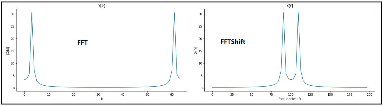
N의 값이 짝(even)일 때 가로 축의 0에서 N-1 까지 범위에 DFT로 계산된 주파수 스펙트럼을 가시화할 수 있다. 하지만 양의(positive) 주파수 값에 해당하는 0~(N/2-1) 과 음의 주파수 값에 해당하는 (N/2)~(N-1) 까지의 모습을 보여주기 때문에 음의 주파수 부분 (N/2)~(N-1)을 가로축 상의 0 즉 DC 성분 값을 중심으로 이동(shift)시켜 가시화 해보자.
• X[1] to X[N/2−1] :양의 값을 가지는주파수 성분들
• X[N/2] : Nyquist 임계 주파수 값 --> 이동
• X[N/2] to X[N −1] : 음의 주파수 값 성분들 --> 이동
음의 값을 가지는 주파수 성분들을 다음그림에서 처럼 이동시키도록 하자.

이와 같이 주파수 스펙트럼 성분 Shift 작업을 코사인 파형을 대상으로 확인해 보자.
DFT에 의해서 얻어진 주파수 스펙트럼을 대상으로 Shift 작업을 하자. 헤더 영역에서 라이브러리 fftshift를 추가하자.
그밖에 ifft 및 ifftshift 는 시계열 파형으로 복하는데 사용하는 라이브러리이다.

"DFT 신호처리 및 AWGN 화이트 노이즈 효과 시각화"에 첨부했던 코드 DFT_Cosine.py 를 일부 수정해서 실행하자.
코사인 파형의 주파수는 10Hz 로 둔다.
DFT 실행 결과를 소문자 x 로 두고 Shift한 결과를 X 로 두자. 소문자 x는 가로축을 N 포인트로 처리하고 대문자 X는 주파수로 처리하기로 한다.

아래에서 Shift 한 결과를 관찰하자. 아울러 주의해야할 점은 역퓨리에 변환 작업을 위해서는 반드시 fft의 결과인 소문자 x 를 사용해야 한다는 점이다. Shfting 한 대문자 X 로는 역 퓨리에 변환이 제대로 안된다는 점에 유의하자.
지금까지는 시계열 데이터를 FFT 변환하여 주파수 스펙트럼을 얻었고 좀 보 보기 좋도록 Shift 작업을 통해서 대칭 형태로 결과를 얻었다. 이와는 반대로 주파수 스펙트럼에서 다시 시계열 데이터로 복귀 시키는 작업을 해 보도록 한다.
ifftshift 는 fft 결과를 shift하여 만들었던 대칭적 결과를 원상 복구하는 명령이다. 원상 복구 후 다시 시계열 데이터로 되돌리기 위해서는 현재 FFT 계산에 사용했던 FFT_size 에 해당하는 N 만큼의 데이터를 사용한다.

복원된 파형이 시산 구간이 변했지만 주어진 코사인 파형이 복원 되었음을 알 수 있다.

코드 해설 유튜브 영상 참조하세요. 구독 좋아요 부탁드려요.
#DFT_Cosine_Shift.py
import numpy as np
from numpy import sum,isrealobj,sqrt
from numpy.random import standard_normal
import matplotlib.pyplot as plt
from scipy.fftpack import fft,ifft
from scipy.fftpack import fftshift, ifftshift
fc = 10 # frequency of the carrier
L = 20 # oversampling factor
fs=L*fc # sampling frequency with oversampling factor
t=np.arange(start = 0,stop = 10,step = 1/fs) # 2 seconds duration
s=np.cos(2*np.pi*fc*t)
# Waveforms at the transmitter
fig0 = plt.figure(figsize=(10,5))
plt.plot(t,s) # baseband wfm zoomed to first 10 bits
plt.xlabel('t(s)');plt.ylabel(r'$s_{bb}(t)$-baseband')
plt.xlim(0,1)
plt.show()
SNRdB = 2
gamma = 10**(SNRdB/10) #SNR to linear scale
P=L*sum(abs(s)**2)/len(s) #Actual power in the vector
N0=P/gamma # Find the noise spectral density
n = sqrt(N0/2)*standard_normal(s.shape)
#s = s + n
# Waveforms at the transmitter
fig1 = plt.figure(figsize=(10,5))
plt.plot(t,s) # baseband wfm zoomed to first 10 bits
plt.xlabel('t(s)');plt.ylabel(r'$s_{bb}(t)$-baseband')
plt.xlim(0,1)
plt.show()
fig2 = plt.figure(figsize=(10,5))
N=64 # FFT size
x = fft(s,N) # N-point complex DFT, output contains DC at index 0
X = fftshift(x)
df=fs/N # frequency resolution
sampleIndex = np.arange(start = 0,stop = N) # raw index for FFT plot
f=sampleIndex*df # x-axis index converted to frequencies
plt.plot(sampleIndex,abs(x))
plt.title('X[k]')
plt.xlabel('k')
plt.ylabel('|X(k)|')
fig3 = plt.figure(figsize=(10,5))
plt.plot(f,abs(X))
plt.title('X[f]')
plt.xlabel('frequencies (f)')
plt.ylabel('|X(f)|')
x_recon = N*ifft(ifftshift(X),N) # reconstructed signal
t = np.arange(start = 0,stop = len(x_recon))/fs # recompute time index
fig4 = plt.figure(figsize=(10,5))
plt.plot(t,np.real(x_recon)) # reconstructed signal
plt.title('reconstructed signal')
plt.xlabel('time (t seconds)')
plt.ylabel('x(t)');
fig4.show()
'통신' 카테고리의 다른 글
| Channel Coding (0) | 2022.04.03 |
|---|---|
| Differential BPSK(DBPSK) 변조 (0) | 2022.03.25 |
| Constellation Diagram 과 QPSK(Quadruple Phase Shift Keying) , QAM(Quadrature Amplitude Modulation) 해설 (0) | 2022.03.24 |
| DFT(Digital Fourier Transform) 신호처리 및 AWGN 화이트 노이즈 시각화 (0) | 2022.03.23 |
| BPSK 변조에서 AGWN(Eb/No)노이즈에 의한 BER 이론 계산 (0) | 2022.03.12 |