BPSK변조 방식에서는 "0"과 "1"로 이루어진 데이터들을 전송을 위해서 2배 후 - 1 하여 "-1"과 "+1" 로 변조하여 carrier에 실어서 전송한다. 특히 시뮬레이션에서는 실제의 전송데이터를 대상으로 하는 것이 아니라 난수 생성 명령을 사용하여 50:50확률로 비율이 조절된 "0"과 "1"로 구성되는 데이터들을 BPSK 시뮬레이션에 사용한다.
반면에 Differential BPSK 변조에서는 아래 그림에서 처럼 "0"과 "1"을 생성함에 있어서 바로 앞 데이터와 위상(phase)이 같은지 여부를 XNOR 논리를 기준으로 따져 결정한다.
즉 "0"&"0" 이거나 "1"&"1" 이면 동일 위상 -> "1"
아니면 "0"&"1" 이거나 "1"&"0" 이면 다른 위상 ->"0"

앞 데이터와 위상(phase)이 같은지 여부를 결정하기 위한 알고리듬을 난수생성 명령과 lfilter 명령을 사용하여 구현하여 보자.
#난수생성 명령 randint을 사용하여 "0"과 "1" 을 N=20개를 생성하자.
ak = np.random.randint(2, size=N) # uniform random symbols from 0's and 1's
# 0 1 2 3 4 5 6 7 8 9...
print(ak) #x[n] -->[0 1 1 1 1 1 0 0 0 1 0 0 1 1 0 0 0 0 1 0]
bk = lfilter([1.0],[1.0,-1.0],ak) # IIR filter for differential encoding
print(bk) #-->[0. 1. 2. 3. 4. 5. 5. 5. 5. 6. 6. 6. 7. 8. 8. 8. 8. 8. 9. 9.]
bk = bk%2 #XOR operation is equivalent to modulo-2
print(bk)
lfilter 명령에 대해서 간단히 알아보자. IIR 필터기능을 수행하는 복잡한 명령이지만 여기서는 앞 데이터와의 위상이 변경되었는지 체크하여 변경되었으면 앞 데이터에 "+1" 만큼 증가시키고 변화가 없으면 "0" 즉 그대로 유지하기로 한다.
y = lfilter( b[0], [ a[0], a[1] ], x )에서 lfilter(+1, [+1, -1], x) 라는 명령을 실행하면 리스트 데이터 x 와 y 사이에 다음과 같은 관계가 얻어진다.
a[0]*y[n] = b[0]*x[n] - b[1]*y[n-1] --> y[n] = x[n] + y[n-1]
즉 y[n] 은 x[n]에 이전 데이터 y[n-1] 을 가산해주게 된다.
y[n-1] 데이터의 초기화는 0으로 두기로 하자:
y[0]=0 & x[0]=0.
x[n=1]=1--> y[n=1]=1+0=1-->y[n=2]=x[2]+y[1]=1+1=2-->y[n=3]=x[3]+y[2]=1+2=3
-->y[n=4]=x[4]+y[3]=1+3=4-->y[n=5]=x[5]+y[4]=1+4=5-->y[n=6]=x[6]+y[5]=0+5=5
-->y[n=6]=x[6]+y[5]=0+5=5-->y[n=7]=x[7]+y[6]=0+5=5-->y[n=8]=x[8]+y[7]=0+5=5
-->y[n=9]=x[9]+y[8]=1+5=6
위 수열에 의한 결과를 정리하면 다음과 같은 리스트 데이터가 얻어진다.
[0. 1. 2. 3. 4. 5. 5. 5. 5. 6. 6. 6. 7. 8. 8. 8. 8. 8. 9. 9.]
이 결과의 의미는 x[n] 의 값 위상이 0-->1로 변경되면 y[n]은 그 이전 값 y[n-1} 대비 +1민큼 증가한다.
아울러 x가 그대로 "+1" 값을 유지하면 y는 계속 "+1"만큼씩 증가하다가 x가 다시 "0'이 되어 지속되면 y는 그대로 값이 유지된다.
lfilter에 의해 얻어진 값들을 %2 로 나누어 나머지를 관찰하고 이 나머지로 리스트 데이터를 만들어 bk로 두자. 이 작업이 바로 XOR 화 작업이다.
bk = [0. 1. 0. 1. 0. 1. 1. 1. 1. 0. 0. 0. 1. 0. 0. 0. 0. 0. 1. 1.]
이 XOR 화 된 데이터를 NRZ (Non Return Zero) 코드화 하여 carrier에 실어서 전송하게 된다. 그 나마지 이어지는 시뮬레이션 코드는 BPSK 코드와 동일하다고 보면 된다. 변조되어 전송된 코드를 복조함에 있어서 앞서의 과정을 역으로 처리하는 알고리듬이 필요할 것이다.
하지만 Differential BPSK 기법은 복조과정에서 2개의 비트 정보를 사용하기 때문에 그 중 어느 하나의 비트가 잘못될 경우 성능이 떨어지게 된다. 즉 앞 비트가 잘못 복조되는 경우와 현재의 비트 정보가 잘못된 2가지 경우가 있을 수 있다. 하나의 비트가 에러일 확률은 BPSK에서 아래와 같이 구해졌다.
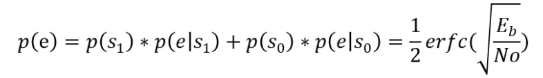
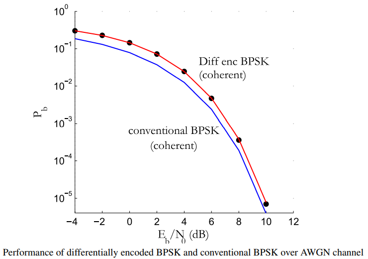
이 공식을 사용하여 Differential BPSK에 적용하면 다음의 BER 공식이 얻어진다. 이 결과는 순수한 BPSK 보다 높은 BER 값을 보여 준다.

Differential BPSK 와 저농적인 BPSK에 의한 BER 값을 EB/n0 파라메터 항으로 아래와 같이 작도해보자. Differential BPSK가 다소 높은 값들을 보여준다.
한편 Differential BPSK에 있어서 변조과정의 역순으로 진행되는 복조(demodulation) 과정은 상당히 복잡할 수도 있다. 왜냐면 복조과정은 변조과정에서 사용했던 정보로서 carrier 주파수와 위상(phase) 정보가 기준정보(reference)로서 반드시 필요하다. 하지만 복조과정에서 사용하는 Costalos loop 또는 PLL(phase Locked loop) 회로에서는 위상정보에 관한 모호성내지는 에러가 발생할 수 있다는 점이다. 위상정보가 -pi 만큼 차이가 나면 아예 값이 반전되어 버릴 수도 있다. 이러한 점을 실용적으로 해결하기 위한 방안으로서 suboptimum 기법과 optimum 기법이 있다. 물론 이 기법들을 사용하면 BER 값이 다소 상승하기는 하나 그만큼 복조회로가 간단해지는 이점이 있을 수 있다는 점을 지적해 둔다.
전통적인 BPSK 즉 Coherent Receiver 에서는 변조에 사용된 정확한 주파수와 위상 정보가 필요하다. 하지만 때로는 이 필수적인 두가지 정보가 결핍된 경우에도 가능한 demodulation 작업 즉 suboptimum BPSK 를 고려해보자.
carrier 주파수에 대한 정확한 값을 모르기때문에 1차적으로 bandpass filter 를 사용하여 신호를 걸른 다음 이 신호호부터 2개의 비트 데이터를 준비해서 적분하여 변조 작업을 실행한다.

Suboptimum DBPSK 의 BER 은 다음과 같이 주어진다.

정확한 carrier 주파수와 위상을 모르는 경우에도 실용적으로 suboptimum 기법이 사용될 수 있을 것이다. 전통적인 BPSK 기법과 suboptimum 사이에 ㅎ당하는 기법으로 optimum 기법은 정확한 carrier 주파수가 주어지는 경우이며 그 BER 은 다음과 같이 주어진다.

첨부된 파일을 다운받아 실행해 보자. dbpsk_noncoherent.py 를 포함하는 폴더 "chapter_2"로 한 레벨 올린 다음
exec(open("chapter_2/dbpsk_noncoherent.py").read()) 명령을 실행해야 한다. 물론 이 폴더 내에 passband_modulations.py와 channels.py 가 포함되어 있어야 한다. 상당히 길이가 긴 passband_modulations.py를 살펴보면 DBPSK 실행에 필요한 부분은 dbpsk_noncoherent 관련 함수 일부이지만 메인 코드 앞 부분에 def 함수로 처리하기에는 다소 긴편이란 점에 유의하자.
#dbpsk_noncoherent.py
#Execute in Python3: exec(open("chapter_2/dbpsk_noncoherent.py").read())
import numpy as np #for numerical computing
import matplotlib.pyplot as plt #for plotting functions
from passband_modulations import bpsk_mod
from channels import awgn
from scipy.signal import lfilter
from scipy.special import erfc
N=100000 # Number of symbols to transmit
EbN0dB = np.arange(start=-4,stop = 11,step = 2) # Eb/N0 range in dB for simulation
L=8 # oversampling factor,L=Tb/Ts(Tb=bit period,Ts=sampling period)
# if a carrier is used, use L = Fs/Fc, where Fs >> 2xFc
Fc=800 # carrier frequency
Fs=L*Fc # sampling frequency
BER_suboptimum = np.zeros(len(EbN0dB)) # BER measures
BER_optimum = np.zeros(len(EbN0dB))
#-----------------Transmitter---------------------
ak = np.random.randint(2, size=N) # uniform random symbols from 0's and 1's
bk = lfilter([1.0],[1.0,-1.0],ak) # IIR filter for differential encoding
bk = bk%2 #XOR operation is equivalent to modulo-2
[s_bb,t]= bpsk_mod(bk,L) # BPSK modulation(waveform) - baseband
s = s_bb*np.cos(2*np.pi*Fc*t/Fs).astype(complex) # DBPSK with carrier
for i,EbN0 in enumerate(EbN0dB):
# Compute and add AWGN noise
r = awgn(s,EbN0,L) # refer Chapter section 4.1
#----------suboptimum receiver---------------
p=np.real(r)*np.cos(2*np.pi*Fc*t/Fs) # demodulate to baseband using BPF
w0= np.hstack((p,np.zeros(L))) # append L samples on one arm for equal lengths
w1= np.hstack((np.zeros(L),p)) # delay the other arm by Tb (L samples)
w = w0*w1 # multiplier
z = np.convolve(w,np.ones(L)) #integrator from kTb to (K+1)Tb (L samples)
u = z[L-1:-1-L:L] # sampler t=kTb
ak_hat = (u<0) #decision
BER_suboptimum[i] = np.sum(ak!=ak_hat)/N #BER for suboptimum receiver
print(BER_suboptimum[i])
#-----------optimum receiver--------------
p=np.real(r)*np.cos(2*np.pi*Fc*t/Fs); # multiply I arm by cos
q=np.imag(r)*np.sin(2*np.pi*Fc*t/Fs) # multiply Q arm by sin
x = np.convolve(p,np.ones(L)) # integrate I-arm by Tb duration (L samples)
y = np.convolve(q,np.ones(L)) # integrate Q-arm by Tb duration (L samples)
xk = x[L-1:-1:L] # Sample every Lth sample
yk = y[L-1:-1:L] # Sample every Lth sample
w0 = xk[0:-2] # non delayed version on I-arm
w1 = xk[1:-1] # 1 bit delay on I-arm
z0 = yk[0:-2] # non delayed version on Q-arm
z1 = yk[1:-1] # 1 bit delay on Q-arm
u =w0*w1 + z0*z1 # decision statistic
ak_hat=(u<0) # threshold detection
BER_optimum[i] = np.sum(ak[1:-1]!=ak_hat)/N # BER for optimum receiver
#------Theoretical Bit/Symbol Error Rates-------------
EbN0lins = 10**(EbN0dB/10) # converting dB values to linear scale
theory_DBPSK_optimum = 0.5*np.exp(-EbN0lins)
theory_DBPSK_suboptimum = 0.5*np.exp(-0.76*EbN0lins)
theory_DBPSK_coherent=erfc(np.sqrt(EbN0lins))*(1-0.5*erfc(np.sqrt(EbN0lins)))
theory_BPSK_conventional = 0.5*erfc(np.sqrt(EbN0lins))
#-------------Plotting---------------------------
fig, ax = plt.subplots(nrows=1,ncols = 1)
ax.semilogy(EbN0dB,BER_suboptimum,'k*',label='DBPSK subopt (sim)')
ax.semilogy(EbN0dB,BER_optimum,'b*',label='DBPSK opt (sim)')
ax.semilogy(EbN0dB,theory_DBPSK_suboptimum,'m-',label='DBPSK subopt (theory)')
ax.semilogy(EbN0dB,theory_DBPSK_optimum,'r-',label='DBPSK opt (theory)')
ax.semilogy(EbN0dB,theory_DBPSK_coherent,'k-',label='coherent DEBPSK')
ax.semilogy(EbN0dB,theory_BPSK_conventional,'b-',label='coherent BPSK')
ax.set_title('Probability of D-BPSK over AWGN')
ax.set_xlabel('$E_b/N_0 (dB)$');ax.set_ylabel('$Probability of Bit Error - P_b$')
ax.legend();fig.show()
#passband_modulations.py
import numpy as np
import matplotlib.pyplot as plt
def bpsk_mod(ak,L):
"""
Function to modulate an incoming binary stream using BPSK (baseband)
Parameters:
ak : input binary data stream (0's and 1's) to modulate
L : oversampling factor (Tb/Ts)
Returns:
(s_bb,t) : tuple of following variables
s_bb: BPSK modulated signal(baseband) - s_bb(t)
t : generated time base for the modulated signal
"""
from scipy.signal import upfirdn
s_bb = upfirdn(h=[1]*L, x=2*ak-1, up = L) # NRZ encoder
t=np.arange(start = 0,stop = len(ak)*L) #discrete time base
return (s_bb,t)
def bpsk_demod(r_bb,L):
"""
Function to demodulate a BPSK (baseband) signal
Parameters:
r_bb : received signal at the receiver front end (baseband)
L : oversampling factor (Tsym/Ts)
Returns:
ak_hat : detected/estimated binary stream
"""
x = np.real(r_bb) #
x = np.convolve(x,np.ones(L)) # integrate for Tb duration (L samples)
x = x[L-1:-1:L] # sample at every L
ak_hat = (x > 0).transpose() # threshold detector
return ak_hat
def add_awgn_noise(s,SNRdB,L=1):
"""
Function to add AWGN noise to input signal
The function adds AWGN noise vector to signal 's' to generate a \
resulting signal vector 'r' of specified SNR in dB. It also returns\
the noise vector 'n' that is added to the signal 's' and the spectral\
density N0 of noise added
Parameters:
s : input/transmitted signal vector
SNRdB : desired signal to noise ratio (expressed in dB)
for the received signal
L : oversampling factor (applicable for waveform simulation)
default L = 1.
Returns:
(r,n,N0) : tuple of following variables
r : received signal vector (r = s+n)
n : noise signal vector added
N0 : spectral density of the generated noise vector n
"""
gamma = 10**(SNRdB/10) #SNR to linear scale
if s.ndim==1:# if s is single dimensional vector
P=L*np.sum(abs(s)**2)/len(s) #Actual power in the vector
else: # multi-dimensional signals like MFSK
P=L*np.sum(np.sum(abs(s)**2))/len(s) # if s is a matrix [MxN]
N0=P/gamma # Find the noise spectral density
from numpy.random import standard_normal
if np.isrealobj(s):# check if input is real/complex object type
n = np.sqrt(N0/2)*standard_normal(s.shape) # computed noise
else:
n = np.sqrt(N0/2)*(standard_normal(s.shape)+1j*standard_normal(s.shape)) #computed noise
r = s + n # received signal
return (r,n,N0)
def qpsk_mod(a, fc, OF, enable_plot = False):
"""
Modulate an incoming binary stream using conventional QPSK
Parameters:
a : input binary data stream (0's and 1's) to modulate
fc : carrier frequency in Hertz
OF : oversampling factor - at least 4 is better
enable_plot : True = plot transmitter waveforms (default False)
Returns:
result : Dictionary containing the following keyword entries:
s(t) : QPSK modulated signal vector with carrier i.e, s(t)
I(t) : baseband I channel waveform (no carrier)
Q(t) : baseband Q channel waveform (no carrier)
t : time base for the carrier modulated signal
"""
L = 2*OF # samples in each symbol (QPSK has 2 bits in each symbol)
I = a[0::2];Q = a[1::2] #even and odd bit streams
# even/odd streams at 1/2Tb baud
from scipy.signal import upfirdn #NRZ encoder
I = upfirdn(h=[1]*L, x=2*I-1, up = L)
Q = upfirdn(h=[1]*L, x=2*Q-1, up = L)
fs = OF*fc # sampling frequency
t=np.arange(0,len(I)/fs,1/fs) #time base
I_t = I*np.cos(2*np.pi*fc*t);Q_t = -Q*np.sin(2*np.pi*fc*t)
s_t = I_t + Q_t # QPSK modulated baseband signal
if enable_plot:
fig = plt.figure(constrained_layout=True)
from matplotlib.gridspec import GridSpec
gs = GridSpec(3, 2, figure=fig)
ax1 = fig.add_subplot(gs[0, 0]);ax2 = fig.add_subplot(gs[0, 1])
ax3 = fig.add_subplot(gs[1, 0]);ax4 = fig.add_subplot(gs[1, 1])
ax5 = fig.add_subplot(gs[-1,:])
# show first few symbols of I(t), Q(t)
ax1.plot(t,I);ax1.set_title('I(t)')
ax2.plot(t,Q);ax2.set_title('Q(t)')
ax3.plot(t,I_t,'r');ax3.set_title('$I(t) cos(2 \pi f_c t)$')
ax4.plot(t,Q_t,'r');ax4.set_title('$Q(t) sin(2 \pi f_c t)$')
ax1.set_xlim(0,20*L/fs);ax2.set_xlim(0,20*L/fs)
ax3.set_xlim(0,20*L/fs);ax4.set_xlim(0,20*L/fs)
ax5.plot(t,s_t);ax5.set_xlim(0,20*L/fs);fig.show()
ax5.set_title('$s(t) = I(t) cos(2 \pi f_c t) - Q(t) sin(2 \pi f_c t)$')
result = dict()
result['s(t)'] =s_t;result['I(t)'] = I;result['Q(t)'] = Q;result['t'] = t
return result
def qpsk_demod(r,fc,OF,enable_plot=False):
"""
Demodulate a conventional QPSK signal
Parameters:
r : received signal at the receiver front end
fc : carrier frequency (Hz)
OF : oversampling factor (at least 4 is better)
enable_plot : True = plot receiver waveforms (default False)
Returns:
a_hat - detected binary stream
"""
fs = OF*fc # sampling frequency
L = 2*OF # number of samples in 2Tb duration
t=np.arange(0,len(r)/fs,1/fs) # time base
x=r*np.cos(2*np.pi*fc*t) # I arm
y=-r*np.sin(2*np.pi*fc*t) # Q arm
x = np.convolve(x,np.ones(L)) # integrate for L (Tsym=2*Tb) duration
y = np.convolve(y,np.ones(L)) #integrate for L (Tsym=2*Tb) duration
x = x[L-1::L] # I arm - sample at every symbol instant Tsym
y = y[L-1::L] # Q arm - sample at every symbol instant Tsym
a_hat = np.zeros(2*len(x))
a_hat[0::2] = (x>0) # even bits
a_hat[1::2] = (y>0) # odd bits
if enable_plot:
fig, axs = plt.subplots(1, 1)
axs.plot(x[0:200],y[0:200],'o');fig.show()
return a_hat
def oqpsk_mod(a,fc,OF,enable_plot=False):
"""
Modulate an incoming binary stream using OQPSK
Parameters:
a : input binary data stream (0's and 1's) to modulate
fc : carrier frequency in Hertz
OF : oversampling factor - at least 4 is better
enable_plot : True = plot transmitter waveforms (default False)
Returns:
result : Dictionary containing the following keyword entries:
s(t) : QPSK modulated signal vector with carrier i.e, s(t)
I(t) : baseband I channel waveform (no carrier)
Q(t) : baseband Q channel waveform (no carrier)
t : time base for the carrier modulated signal
"""
L = 2*OF # samples in each symbol (QPSK has 2 bits in each symbol)
I = a[0::2];Q = a[1::2] #even and odd bit streams
# even/odd streams at 1/2Tb baud
from scipy.signal import upfirdn #NRZ encoder
I = upfirdn(h=[1]*L, x=2*I-1, up = L)
Q = upfirdn(h=[1]*L, x=2*Q-1, up = L)
I = np.hstack((I,np.zeros(L//2))) # padding at end
Q = np.hstack((np.zeros(L//2),Q)) # padding at start
fs = OF*fc # sampling frequency
t=np.arange(0,len(I)/fs,1/fs) #time base
I_t = I*np.cos(2*np.pi*fc*t);Q_t = -Q*np.sin(2*np.pi*fc*t)
s = I_t + Q_t # QPSK modulated baseband signal
if enable_plot:
fig = plt.figure(constrained_layout=True)
from matplotlib.gridspec import GridSpec
gs = GridSpec(3, 2, figure=fig)
ax1 = fig.add_subplot(gs[0, 0]);ax2 = fig.add_subplot(gs[0, 1])
ax3 = fig.add_subplot(gs[1, 0]);ax4 = fig.add_subplot(gs[1, 1])
ax5 = fig.add_subplot(gs[-1,:])
# show first few symbols of I(t), Q(t)
ax1.plot(t,I);ax1.set_title('I(t)')
ax2.plot(t,Q);ax2.set_title('Q(t)')
ax3.plot(t,I_t,'r');ax3.set_title('$I(t) cos(2 \pi f_c t)$')
ax4.plot(t,Q_t,'r');ax4.set_title('$Q(t) sin(2 \pi f_c t)$')
ax1.set_xlim(0,20*L/fs);ax2.set_xlim(0,20*L/fs)
ax3.set_xlim(0,20*L/fs);ax4.set_xlim(0,20*L/fs)
ax5.plot(t,s);ax5.set_xlim(0,20*L/fs);fig.show()
ax5.set_title('$s(t) = I(t) cos(2 \pi f_c t) - Q(t) sin(2 \pi f_c t)$')
fig, axs = plt.subplots(1, 1)
axs.plot(I,Q);fig.show()#constellation plot
result = dict()
result['s(t)'] =s;result['I(t)'] = I;result['Q(t)'] = Q;result['t'] = t
return result
def oqpsk_demod(r,N,fc,OF,enable_plot=False):
"""
Demodulate a OQPSK signal
Parameters:
r : received signal at the receiver front end
N : Number of OQPSK symbols transmitted
fc : carrier frequency (Hz)
OF : oversampling factor (at least 4 is better)
enable_plot : True = plot receiver waveforms (default False)
Returns:
a_hat - detected binary stream
"""
fs = OF*fc # sampling frequency
L = 2*OF # number of samples in 2Tb duration
t=np.arange(0,(N+1)*OF/fs,1/fs) # time base
x=r*np.cos(2*np.pi*fc*t) # I arm
y=-r*np.sin(2*np.pi*fc*t) # Q arm
x = np.convolve(x,np.ones(L)) # integrate for L (Tsym=2*Tb) duration
y = np.convolve(y,np.ones(L)) #integrate for L (Tsym=2*Tb) duration
x = x[L-1:-1-L:L] # I arm - sample at every symbol instant Tsym
y = y[L+L//2-1:-1-L//2:L] # Q arm - sample at every symbol starting at L+L/2-1th sample
a_hat = np.zeros(N)
a_hat[0::2] = (x>0) # even bits
a_hat[1::2] = (y>0) # odd bits
if enable_plot:
fig, axs = plt.subplots(1, 1)
axs.plot(x[0:200],y[0:200],'o');fig.show()
return a_hat
def piBy4_dqpsk_Diff_encoding(a,enable_plot=False):
"""
Phase Mapper for pi/4-DQPSK modulation
Parameters:
a : input stream of binary bits
Returns:
(u,v): tuple, where
u : differentially coded I-channel bits
v : differentially coded Q-channel bits
"""
from numpy import pi, cos, sin
if len(a)%2: raise ValueError('Length of binary stream must be even')
I = a[0::2] # odd bit stream
Q = a[1::2] # even bit stream
# club 2-bits to form a symbol and use it as index for dTheta table
m = 2*I+Q
dTheta = np.array([-3*pi/4, 3*pi/4, -pi/4, pi/4]) #LUT for pi/4-DQPSK
u = np.zeros(len(m)+1);v = np.zeros(len(m)+1)
u[0]=1; v[0]=0 # initial conditions for uk and vk
for k in range(0,len(m)):
u[k+1] = u[k] * cos(dTheta[m[k]]) - v[k] * sin(dTheta[m[k]])
v[k+1] = u[k] * sin(dTheta[m[k]]) + v[k] * cos(dTheta[m[k]])
if enable_plot:#constellation plot
fig, axs = plt.subplots(1, 1)
axs.plot(u,v,'o');
axs.set_title('Constellation');fig.show()
return (u,v)
def piBy4_dqpsk_mod(a,fc,OF,enable_plot = False):
"""
Modulate a binary stream using pi/4 DQPSK
Parameters:
a : input binary data stream (0's and 1's) to modulate
fc : carrier frequency in Hertz
OF : oversampling factor
Returns:
result : Dictionary containing the following keyword entries:
s(t) : pi/4 QPSK modulated signal vector with carrier
U(t) : differentially coded I-channel waveform (no carrier)
V(t) : differentially coded Q-channel waveform (no carrier)
t: time base
"""
(u,v)=piBy4_dqpsk_Diff_encoding(a) # Differential Encoding for pi/4 QPSK
#Waveform formation (similar to conventional QPSK)
L = 2*OF # number of samples in each symbol (QPSK has 2 bits/symbol)
U = np.tile(u, (L,1)).flatten('F')# odd bit stream at 1/2Tb baud
V = np.tile(v, (L,1)).flatten('F')# even bit stream at 1/2Tb baud
fs = OF*fc # sampling frequency
t=np.arange(0, len(U)/fs,1/fs) #time base
U_t = U*np.cos(2*np.pi*fc*t)
V_t = -V*np.sin(2*np.pi*fc*t)
s_t = U_t + V_t
if enable_plot:
fig = plt.figure(constrained_layout=True)
from matplotlib.gridspec import GridSpec
gs = GridSpec(3, 2, figure=fig)
ax1 = fig.add_subplot(gs[0, 0]);ax2 = fig.add_subplot(gs[0, 1])
ax3 = fig.add_subplot(gs[1, 0]);ax4 = fig.add_subplot(gs[1, 1])
ax5 = fig.add_subplot(gs[-1,:])
ax1.plot(t,U);ax2.plot(t,V)
ax3.plot(t,U_t,'r');ax4.plot(t,V_t,'r')
ax5.plot(t,s_t) #QPSK waveform zoomed to first few symbols
ax1.set_ylabel('U(t)-baseband');ax2.set_ylabel('V(t)-baseband')
ax3.set_ylabel('U(t)-with carrier');ax4.set_ylabel('V(t)-with carrier')
ax5.set_ylabel('s(t)');ax5.set_xlim([0,10*L/fs])
ax1.set_xlim([0,10*L/fs]);ax2.set_xlim([0,10*L/fs])
ax3.set_xlim([0,10*L/fs]);ax4.set_xlim([0,10*L/fs])
fig.show()
result = dict()
result['s(t)'] =s_t;result['U(t)'] = U;result['V(t)'] = V;result['t'] = t
return result
def piBy4_dqpsk_Diff_decoding(w,z):
"""
Phase Mapper for pi/4-DQPSK modulation
Parameters:
w - differentially coded I-channel bits at the receiver
z - differentially coded Q-channel bits at the receiver
Returns:
a_hat - binary bit stream after differential decoding
"""
if len(w)!=len(z): raise ValueError('Length mismatch between w and z')
x = np.zeros(len(w)-1);y = np.zeros(len(w)-1);
for k in range(0,len(w)-1):
x[k] = w[k+1]*w[k] + z[k+1]*z[k]
y[k] = z[k+1]*w[k] - w[k+1]*z[k]
a_hat = np.zeros(2*len(x))
a_hat[0::2] = (x > 0) # odd bits
a_hat[1::2] = (y > 0) # even bits
return a_hat
def piBy4_dqpsk_demod(r,fc,OF,enable_plot=False):
"""
Differential coherent demodulation of pi/4-DQPSK
Parameters:
r : received signal at the receiver front end
fc : carrier frequency in Hertz
OF : oversampling factor (multiples of fc) - at least 4 is better
Returns:
a_cap : detected binary stream
"""
fs = OF*fc # sampling frequency
L = 2*OF # samples in 2Tb duration
t=np.arange(0, len(r)/fs,1/fs)
w=r*np.cos(2*np.pi*fc*t) # I arm
z=-r*np.sin(2*np.pi*fc*t) # Q arm
w = np.convolve(w,np.ones(L)) # integrate for L (Tsym=2*Tb) duration
z = np.convolve(z,np.ones(L)) # integrate for L (Tsym=2*Tb) duration
w = w[L-1::L] # I arm - sample at every symbol instant Tsym
z = z[L-1::L] # Q arm - sample at every symbol instant Tsym
a_cap = piBy4_dqpsk_Diff_decoding(w,z)
if enable_plot:#constellation plot
fig, axs = plt.subplots(1, 1)
axs.plot(w,z,'o')
axs.set_title('Constellation');fig.show()
return a_cap
def msk_mod(a, fc, OF, enable_plot = False):
"""
Modulate an incoming binary stream using MSK
Parameters:
a : input binary data stream (0's and 1's) to modulate
fc : carrier frequency in Hertz
OF : oversampling factor (at least 4 is better)
Returns:
result : Dictionary containing the following keyword entries:
s(t) : MSK modulated signal with carrier
sI(t) : baseband I channel waveform(no carrier)
sQ(t) : baseband Q channel waveform(no carrier)
t: time base
"""
ak = 2*a-1 # NRZ encoding 0-> -1, 1->+1
ai = ak[0::2]; aq = ak[1::2] # split even and odd bit streams
L = 2*OF # represents one symbol duration Tsym=2xTb
#upsample by L the bits streams in I and Q arms
from scipy.signal import upfirdn, lfilter
ai = upfirdn(h=[1], x=ai, up = L)
aq = upfirdn(h=[1], x=aq, up = L)
aq = np.pad(aq, (L//2,0), 'constant') # delay aq by Tb (delay by L/2)
ai = np.pad(ai, (0,L//2), 'constant') # padding at end to equal length of Q
#construct Low-pass filter and filter the I/Q samples through it
Fs = OF*fc;Ts = 1/Fs;Tb = OF*Ts
t = np.arange(0,2*Tb+Ts,Ts)
h = np.sin(np.pi*t/(2*Tb))# LPF filter
sI_t = lfilter(b = h, a = [1], x = ai) # baseband I-channel
sQ_t = lfilter(b = h, a = [1], x = aq) # baseband Q-channel
t=np.arange(0, Ts*len(sI_t), Ts) # for RF carrier
sIc_t = sI_t*np.cos(2*np.pi*fc*t) #with carrier
sQc_t = sQ_t*np.sin(2*np.pi*fc*t) #with carrier
s_t = sIc_t - sQc_t# Bandpass MSK modulated signal
if enable_plot:
fig, (ax1,ax2,ax3) = plt.subplots(3, 1)
ax1.plot(t,sI_t);ax1.plot(t,sIc_t,'r')
ax2.plot(t,sQ_t);ax2.plot(t,sQc_t,'r')
ax3.plot(t,s_t,'--')
ax1.set_ylabel('$s_I(t)$');ax2.set_ylabel('$s_Q(t)$')
ax3.set_ylabel('s(t)')
ax1.set_xlim([-Tb,20*Tb]);ax2.set_xlim([-Tb,20*Tb])
ax3.set_xlim([-Tb,20*Tb])
fig.show()
result = dict()
result['s(t)'] =s_t;result['sI(t)'] = sI_t;result['sQ(t)'] = sQ_t;result['t'] = t
return result
def msk_demod(r,N,fc,OF):
"""
MSK demodulator
Parameters:
r : received signal at the receiver front end
N : number of symbols transmitted
fc : carrier frequency in Hertz
OF : oversampling factor (at least 4 is better)
Returns:
a_hat : detected binary stream
"""
L = 2*OF # samples in 2Tb duration
Fs=OF*fc;Ts=1/Fs;Tb = OF*Ts; # sampling frequency, durations
t=np.arange(-OF, len(r) - OF)/Fs # time base
# cosine and sine functions for half-sinusoid shaping
x=abs(np.cos(np.pi*t/(2*Tb)));y=abs(np.sin(np.pi*t/(2*Tb)))
u=r*x*np.cos(2*np.pi*fc*t) # multiply I by half cosines and cos(2pifct)
v=-r*y*np.sin(2*np.pi*fc*t) # multiply Q by half sines and sin(2pifct)
iHat = np.convolve(u,np.ones(L)) # integrate for L (Tsym=2*Tb) duration
qHat = np.convolve(v,np.ones(L)) # integrate for L (Tsym=2*Tb) duration
iHat= iHat[L-1:-1-L:L] # I- sample at the end of every symbol
qHat= qHat[L+L//2-1:-1-L//2:L] # Q-sample from L+L/2th sample
a_hat = np.zeros(N)
a_hat[0::2] = iHat > 0 # thresholding - odd bits
a_hat[1::2] = qHat > 0 # thresholding - even bits
return a_hat
def gaussianLPF(BT, Tb, L, k):
"""
Function to generate filter coefficients of Gaussian low pass filter (used in gmsk_mod)
Parameters:
BT : BT product - Bandwidth x bit period
Tb : bit period
L : oversampling factor (number of samples per bit)
k : span length of the pulse (bit interval)
Returns:
h_norm : normalized filter coefficients of Gaussian LPF
"""
B = BT/Tb # bandwidth of the filter
t = np.arange(start = -k*Tb, stop = k*Tb + Tb/L, step = Tb/L) # truncated time limits for the filter
h = B*np.sqrt(2*np.pi/(np.log(2)))*np.exp(-2 * (t*np.pi*B)**2 /(np.log(2)))
h_norm=h/np.sum(h)
return h_norm
def gmsk_mod(a,fc,L,BT,enable_plot=False):
"""
Function to modulate a binary stream using GMSK modulation
Parameters:
BT : BT product (bandwidth x bit period) for GMSK
a : input binary data stream (0's and 1's) to modulate
fc : RF carrier frequency in Hertz
L : oversampling factor
enable_plot: True = plot transmitter waveforms (default False)
Returns:
(s_t,s_complex) : tuple containing the following variables
s_t : GMSK modulated signal with carrier s(t)
s_complex : baseband GMSK signal (I+jQ)
"""
from scipy.signal import upfirdn,lfilter
fs = L*fc; Ts=1/fs;Tb = L*Ts; # derived waveform timing parameters
c_t = upfirdn(h=[1]*L, x=2*a-1, up = L) #NRZ pulse train c(t)
k=1 # truncation length for Gaussian LPF
h_t = gaussianLPF(BT,Tb,L,k) # Gaussian LPF with BT=0.25
b_t = np.convolve(h_t,c_t,'full') # convolve c(t) with Gaussian LPF to get b(t)
bnorm_t = b_t/max(abs(b_t)) # normalize the output of Gaussian LPF to +/-1
h = 0.5;
phi_t = lfilter(b = [1], a = [1,-1], x = bnorm_t*Ts) * h*np.pi/Tb # integrate to get phase information
I = np.cos(phi_t)
Q = np.sin(phi_t) # cross-correlated baseband I/Q signals
s_complex = I - 1j*Q # complex baseband representation
t = Ts* np.arange(start = 0, stop = len(I)) # time base for RF carrier
sI_t = I*np.cos(2*np.pi*fc*t); sQ_t = Q*np.sin(2*np.pi*fc*t)
s_t = sI_t - sQ_t # s(t) - GMSK with RF carrier
if enable_plot:
fig, axs = plt.subplots(2, 4)
axs[0,0].plot(np.arange(0,len(c_t))*Ts,c_t);axs[0,0].set_title('c(t)');axs[0,0].set_xlim(0,40*Tb)
axs[0,1].plot(np.arange(-k*Tb,k*Tb+Ts,Ts),h_t);axs[0,1].set_title('$h(t): BT_b$='+str(BT))
axs[0,2].plot(t,I,'--');axs[0,2].plot(t,sI_t,'r');axs[0,2].set_title('$I(t)cos(2 \pi f_c t)$');axs[0,2].set_xlim(0,10*Tb)
axs[0,3].plot(t,Q,'--');axs[0,3].plot(t,sQ_t,'r');axs[0,3].set_title('$Q(t)sin(2 \pi f_c t)$');axs[0,3].set_xlim(0,10*Tb)
axs[1,0].plot( np.arange(0,len(bnorm_t))*Ts,bnorm_t);axs[1,0].set_title('b(t)');axs[1,0].set_xlim(0,40*Tb)
axs[1,1].plot(np.arange(0,len(phi_t))*Ts, phi_t);axs[1,1].set_title('$\phi(t)$')
axs[1,2].plot(t,s_t);axs[1,2].set_title('s(t)');axs[1,2].set_xlim(0,20*Tb)
axs[1,3].plot(I,Q);axs[1,3].set_title('constellation')
fig.show()
return (s_t,s_complex)
def gmsk_demod(r_complex,L):
"""
Function to demodulate a baseband GMSK signal
Parameters:
r_complex : received signal at receiver front end (complex form - I+jQ)
L : oversampling factor
Returns:
a_hat : detected binary stream
"""
I=np.real(r_complex); Q = -np.imag(r_complex); # I,Q streams
z1 = Q * np.hstack((np.zeros(L), I[0:len(I)-L]))
z2 = I * np.hstack((np.zeros(L), Q[0:len(I)-L]))
z = z1 - z2
a_hat = (z[2*L-1:-L:L] > 0).astype(int) # sampling and hard decision
#sampling indices depends on the truncation length (k) of Gaussian LPF defined in the modulator
return a_hat
def bfsk_mod(a,fc,fd,L,fs,fsk_type='coherent',enable_plot = False):
"""
Function to modulate an incoming binary stream using BFSK
Parameters:
a : input binary data stream (0's and 1's) to modulate
fc : center frequency of the carrier in Hertz
fd : frequency separation measured from Fc
L : number of samples in 1-bit period
fs : Sampling frequency for discrete-time simulation
fsk_type : 'coherent' (default) or 'noncoherent' FSK generation
enable_plot: True = plot transmitter waveforms (default False)
Returns:
(s_t,phase) : tuple containing following parameters
s_t : BFSK modulated signal
phase : initial phase generated by modulator, applicable only for coherent FSK. It can be used when using coherent detection at Rx
"""
from scipy.signal import upfirdn
a_t = upfirdn(h=[1]*L, x=a, up = L) #data to waveform
t = np.arange(start=0,stop=len(a_t))/fs #time base
if fsk_type.lower() == 'noncoherent':
c1 = np.cos(2*np.pi*(fc+fd/2)*t+2*np.pi*np.random.random_sample()) # carrier 1 with random phase
c2 = np.cos(2*np.pi*(fc-fd/2)*t+2*np.pi*np.random.random_sample()) # carrier 2 with random phase
else: #coherent is default
phase=2*np.pi*np.random.random_sample() # random phase from uniform distribution [0,2pi)
c1 = np.cos(2*np.pi*(fc+fd/2)*t+phase) # carrier 1 with random phase
c2 = np.cos(2*np.pi*(fc-fd/2)*t+phase) # carrier 2 with the same random phase
s_t = a_t*c1 +(-a_t+1)*c2 # BFSK signal (MUX selection)
if enable_plot:
fig, (ax1,ax2) = plt.subplots(2, 1)
ax1.plot(t,a_t);ax2.plot(t,s_t);fig.show()
return (s_t,phase)
def bfsk_coherent_demod(r_t,phase,fc,fd,L,fs):
"""
Coherent demodulation of BFSK modulated signal
Parameters:
r_t : BFSK modulated signal at the receiver r(t)
phase : initial phase generated at the transmitter
fc : center frequency of the carrier in Hertz
fd : frequency separation measured from Fc
L : number of samples in 1-bit period
fs : Sampling frequency for discrete-time simulation
Returns:
a_hat : data bits after demodulation
"""
t = np.arange(start=0,stop=len(r_t))/fs # time base
x = r_t*(np.cos(2*np.pi*(fc+fd/2)*t+phase)-np.cos(2*np.pi*(fc-fd/2)*t+phase))
y = np.convolve(x,np.ones(L)) # integrate/sum from 0 to L
a_hat = (y[L-1::L]>0).astype(int) # sample at every sampling instant and detect
return a_hat
def bfsk_noncoherent_demod(r_t,fc,fd,L,fs):
"""
Non-coherent demodulation of BFSK modulated signal
Parameters:
r_t : BFSK modulated signal at the receiver r(t)
fc : center frequency of the carrier in Hertz
fd : frequency separation measured from Fc
L : number of samples in 1-bit period
fs : Sampling frequency for discrete-time simulation
Returns:
a_hat : data bits after demodulation
"""
t = np.arange(start=0,stop=len(r_t))/fs # time base
f1 = (fc+fd/2); f2 = (fc-fd/2)
#define four basis functions
p1c = np.cos(2*np.pi*f1*t); p2c = np.cos(2*np.pi*f2*t)
p1s = -1*np.sin(2*np.pi*f1*t); p2s = -1*np.sin(2*np.pi*f2*t)
# multiply and integrate from 0 to L
r1c = np.convolve(r_t*p1c,np.ones(L)); r2c = np.convolve(r_t*p2c,np.ones(L))
r1s = np.convolve(r_t*p1s,np.ones(L)); r2s = np.convolve(r_t*p2s,np.ones(L))
# sample at every sampling instant
r1c = r1c[L-1::L]; r2c = r2c[L-1::L]
r1s = r1s[L-1::L]; r2s = r2s[L-1::L]
# square and add
x = r1c**2 + r1s**2
y = r2c**2 + r2s**2
a_hat=((x-y)>0).astype(int) # compare and decide
return a_hat
#channels.py
from numpy import sum,isrealobj,sqrt
from numpy.random import standard_normal
def awgn(s,SNRdB,L=1):
"""
AWGN channel
Add AWGN noise to input signal. The function adds AWGN noise vector to signal
's' to generate a resulting signal vector 'r' of specified SNR in dB. It also
returns the noise vector 'n' that is added to the signal 's' and the power
spectral density N0 of noise added
Parameters:
s : input/transmitted signal vector
SNRdB : desired signal to noise ratio (expressed in dB)
for the received signal
L : oversampling factor (applicable for waveform simulation)
default L = 1.
Returns:
r : received signal vector (r=s+n)
"""
gamma = 10**(SNRdB/10) #SNR to linear scale
if s.ndim==1:# if s is single dimensional vector
P=L*sum(abs(s)**2)/len(s) #Actual power in the vector
else: # multi-dimensional signals like MFSK
P=L*sum(sum(abs(s)**2))/len(s) # if s is a matrix [MxN]
N0=P/gamma # Find the noise spectral density
if isrealobj(s):# check if input is real/complex object type
n = sqrt(N0/2)*standard_normal(s.shape) # computed noise
#n = 1.0*standard_normal(s.shape)
else:
n = sqrt(N0/2)*(standard_normal(s.shape)+1j*standard_normal(s.shape))
r = s + n # received signal
#r = s + 0.1*n
return r
def rayleighFading(N):
"""
Generate Rayleigh flat-fading channel samples
Parameters:
N : number of samples to generate
Returns:
abs_h : Rayleigh flat fading samples
"""
# 1 tap complex gaussian filter
h = 1/sqrt(2)*(standard_normal(N)+1j*standard_normal(N))
return abs(h)
def ricianFading(K_dB,N):
"""
Generate Rician flat-fading channel samples
Parameters:
K_dB: Rician K factor in dB scale
N : number of samples to generate
Returns:
abs_h : Rician flat fading samples
"""
K = 10**(K_dB/10) # K factor in linear scale
mu = sqrt(K/(2*(K+1))) # mean
sigma = sqrt(1/(2*(K+1))) # sigma
h = (sigma*standard_normal(N)+mu)+1j*(sigma*standard_normal(N)+mu)
return abs(h)
Under Construction ...
'통신' 카테고리의 다른 글
| FFTShift & 파형 복구 (0) | 2022.04.05 |
|---|---|
| Channel Coding (0) | 2022.04.03 |
| Constellation Diagram 과 QPSK(Quadruple Phase Shift Keying) , QAM(Quadrature Amplitude Modulation) 해설 (0) | 2022.03.24 |
| DFT(Digital Fourier Transform) 신호처리 및 AWGN 화이트 노이즈 시각화 (0) | 2022.03.23 |
| BPSK 변조에서 AGWN(Eb/No)노이즈에 의한 BER 이론 계산 (0) | 2022.03.12 |