헤더 영역에 필요한 라이브러리들을 선언하자.
| 1 | import os import tensorflow as tf from keras.models import Sequential from keras.layers import Dense, Dropout, Flatten from keras.constraints import maxnorm from keras.optimizers import Adam from keras.layers.convolutional import Conv2D from keras.layers.convolutional import MaxPooling2D from keras.utils import np_utils import numpy as np import time import matplotlib.pyplot as plt |
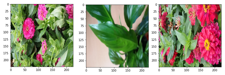
DataSet 폴더로 설정되는 data_root 폴더는 6종의 식물 및 꽃 이미지 폴더들이 들어 있다. 아울러 6종의 폴더명은 라벨값으로 읽힌다.
이미지 폭과 높이는 스마트폰 해상도인 (1152, 2048) 의 반에 해당한다. 이 해상도는 현재 상당히 높은 편이며 어느정도 줄여도 인식률에 큰 영향을 미치지 못한다. 하지만 CNN 신경망 구성 시에 축소되는 이미지 해상도 값을 못 맞춰주면 연산 에러가 발생할 수도 있음에 유의하자. 대안으로 이미지 자체는 좀 왜곡될지라도 254x254 또는 224x224 를 사용하도록 하자.
| 2 | plt.figure() data_root = ("D:/아두이노자료_17_03_24/인공지능응용공학/ImageClassfication/DataSet") img_height = 254 img_width = 254 batch_size = 15 data_dir = str(data_root) |
utils.image_dataset_from_directory 명령을 사용 학습용과 검증용 tf.data.Data 에 해당하는 데이터세트를 준비한다.
| 3 | train_ds = tf.keras.utils.image_dataset_from_directory( data_dir, validation_split=0.2, subset="training", seed=123, image_size=(img_height, img_width), batch_size=batch_size) val_ds = tf.keras.utils.image_dataset_from_directory( data_dir, validation_split=0.2, subset="validation", seed=123, image_size=(img_height, img_width), batch_size=batch_size) |
학습용 데이터세트로부터 포함되어 있는 6종의 식물 라벨값을 class_names 로 출력한다.
학습용 데이터세트로부터 이미지와 라벨값으로 이루어진 튜플 데이터를 설정한다.
| 4 | class_names = train_ds.class_names print(class_names) for image_batch, label_batch in train_ds: print(image_batch.shape) print(label_batch.shape) break for valid_image_batch, valid_label_batch in val_ds: print(valid_image_batch.shape) print(valid_label_batch.shape) break |
이미지 픽셀 데이터 값을 (1/255.)로 리스케일링한다.
normalized_ds 로부터 다음 batch 데이터를 불러와 튜플 데이터로 처리한다.
batch 이미지 데이터 중 첫 번째를 대상으로 픽셀 값의 최소값과 최대 값을 출력해 본다.
| 5 | normalization_layer = tf.keras.layers.Rescaling(1./255) normalized_ds = train_ds.map(lambda x, y: (normalization_layer(x), y)) image_batch, labels_batch = next(iter(normalized_ds)) first_image = image_batch[0] # Notice the pixel values are now in `[0,1]`. print(np.min(first_image), np.max(first_image)) |
학습시킬 식물의 종류 수 즉 라벨 수를 지정한다. 이 수는 utils.image_dataset_from _directory 명령으로 읽어 들이는 폴더 수와 정확하게 일치해야 한다.
CNN 과 완전연결층으로 이루어진 Sequential 신경망 모델을 구성한다.
옵티마이져를 지정하고 Cost 함수를 선정하여 컴파일한다.
| 6 | num_classes = 6 model = tf.keras.Sequential([ tf.keras.layers.Rescaling(1./255), tf.keras.layers.Conv2D(32, 3, activation='relu'), tf.keras.layers.MaxPooling2D(), tf.keras.layers.Conv2D(32, 3, activation='relu'), tf.keras.layers.MaxPooling2D(), tf.keras.layers.Conv2D(32, 3, activation='relu'), tf.keras.layers.MaxPooling2D(), tf.keras.layers.Flatten(), tf.keras.layers.Dense(128, activation='relu'), tf.keras.layers.Dense(num_classes) ]) model.compile( optimizer='adam', loss=tf.keras.losses.SparseCategoricalCrossentropy(from_logits=True), metrics=['accuracy']) |
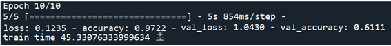
epochs=10 으로 두고 학습을 시킨 후 학습에 걸린 소요시간을 출력해 보자.
| 7 | start = time.time() history = model.fit( train_ds, validation_data=val_ds, epochs=10) end = time.time() print('train time', end-start, '초') |
학습 결과 다음과 같은 출력을 볼 수 있다.
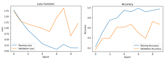
history 명령을 사용하여 Cost 함수와 accuracy 를 작도해 보자.
| 8 | # Plot the loss function plt.figure(figsize=(6, 4)) plt.plot(history.history['loss'], label='Training Loss') plt.plot(history.history['val_loss'], label='Validation Loss') plt.title('Loss Function') plt.xlabel('Epoch') plt.ylabel('Loss') plt.legend() plt.show() # Plot the accuracy plt.figure(figsize=(6, 4)) plt.plot(history.history['accuracy'], label='Training Accuracy') plt.plot(history.history['val_accuracy'], label='Validation Accuracy') plt.title('Accuracy') plt.xlabel('Epoch') plt.ylabel('Accuracy') plt.legend() plt.show() |
Loss 함수와 Accuracy 출력 결과를 살펴보자.
첨부된 파일을 다운받아 epochs를 10에서 20 으로 변경하여 실행해 보자.
'인공지능 응용 공학' 카테고리의 다른 글
| OpenCV 명령을 응용한 하네스 커넥터 확대 이미지의 의 윤곽선 추출 (0) | 2023.06.07 |
|---|---|
| Keras 학습가중치 callback 업로딩에 의한 이미지 분류 (0) | 2023.06.07 |
| 학습가중치 저장 및 업로딩에 의한 Keras MNIST 수기문자 판독 (0) | 2023.06.03 |
| 지적재산기반 인공지능응용 공학 목차 PDF 파일 (0) | 2023.03.05 |
| 지적재산기반 인공지능응용 공학 목차 PDF 파일 (0) | 2023.02.22 |