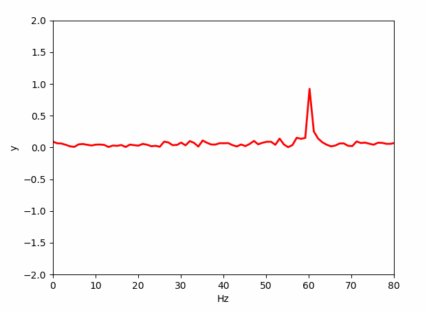
Time domain 상에서 단순 정현파 형태의 파형 디스플레이를 넘어 정현파의 FFT (Fast Fourier Transform)처리에 의한 주파수 분포를 오실로스코프 처럼 애니메이션 해보자. 문제를 간단히 하기 위해서 60HZ 주파수의 정현파와 약간의 노이즈를 섞어 오실스코프 처럼 애니메이션 해보자.
헤더 영역에 필요한 라이러리들을 불러 들인다.
import numpy as np
from matplotlib import pyplot as plt
from matplotlib import animation
from matplotlib.animation import FuncAnimation, PillowWriter
import math
초기화 함수 init()은 animation.Funcanimation 에서 사용된다.
# initialization function: plot the background of each frame
def init():
line.set_data([], [])
return line,
애니메이션 함수 animate(i)는 animation.Funcanimation 에서 사용된다.
이 루틴안에서 정현파 함수를 계산함과 아울러 Time domain 상에서 0.01*i 만큼씩 시간을 진행시키면서 지속적으로 FFT 루틴에 의해 주파수 스펙트럼을 계산한다. Fs=300은 샘플링 갯수이며 t=300 은 샘플링 구간을 뜻한다.
# animation function. This is called sequentially
def animate(i):
Fs = 300
t= 300
x = np.linspace(0, t, Fs)
z = x
noise = np.random.normal(0,0.05,len(x))
y = np.sin(2 * np.pi * 60 * (x - 0.01 * i)) + 10.0 * noise
#+ 0.5 * np.sin(20 * np.pi * 120 * (x - 0.01 * i))
# Calculate FFT ....................
n=len(y) # Length of signal
NFFT=n # ?? NFFT=2^nextpow2(length(y)) ??
k=np.arange(NFFT)
f0=k*Fs/NFFT # double sides frequency range
f0=f0[range(math.trunc(NFFT/2))] # single sied frequency range
Y = np.fft.fft(y)/NFFT # fft computing and normaliation
y = y[range(math.trunc(NFFT/2))]
z = x[range(math.trunc(NFFT/2))]
Y=Y[range(math.trunc(NFFT/2))] # single sied frequency range
amplitude_Hz = 2*abs(Y)
phase_ang = np.angle(Y)*180/np.pi
#line.set_data(z, y)
line.set_data(z, amplitude_Hz)
return line,
함수 init()과 animate(i)가 준비되었으면 그래프 프렘임을 작도하고 2차원 선그래프 형태의 스펙트럼 애니메이션을 시킨다.
fig = plt.figure(num=1, dpi=100, facecolor='white')
ax = plt.axes(xlim=(0, 80), ylim=(-2, 2))
line, = ax.plot([], [], lw=2,color='red')
plt.xlabel('Hz')
plt.ylabel('y')
# call the animator. blit=True means only re-draw the parts that have changed.
anim = animation.FuncAnimation(fig, animate, init_func=init, frames=200, interval=20, blit=True)
아나콘다 프롬프트 창에서 현재의 파이선 코드를 command line 명령 방식으로 실행시켜 gif인 파일을 얻는다.
아래의 gif 파일을 다운받아 열기 하면 애니메이션을 볼 수 있다.
# save the animation as mp4 video file
anim.save('spectrum.gif',writer='matplotlib.animation.PillowWriter')
#spectrum_animation.py
import numpy as np
from matplotlib import pyplot as plt
from matplotlib import animation
from matplotlib.animation import FuncAnimation, PillowWriter
import math
# initialization function: plot the background of each frame
def init():
line.set_data([], [])
return line,
# animation function. This is called sequentially
def animate(i):
Fs = 300
t= 300
x = np.linspace(0, t, Fs)
z = x
noise = np.random.normal(0,0.05,len(x))
y = np.sin(2 * np.pi * 60 * (x - 0.01 * i)) + 10.0 * noise
#+ 0.5 * np.sin(20 * np.pi * 120 * (x - 0.01 * i))
# Calculate FFT ....................
n=len(y) # Length of signal
NFFT=n # ?? NFFT=2^nextpow2(length(y)) ??
k=np.arange(NFFT)
f0=k*Fs/NFFT # double sides frequency range
f0=f0[range(math.trunc(NFFT/2))] # single sied frequency range
Y = np.fft.fft(y)/NFFT # fft computing and normaliation
y = y[range(math.trunc(NFFT/2))]
z = x[range(math.trunc(NFFT/2))]
Y=Y[range(math.trunc(NFFT/2))] # single sied frequency range
amplitude_Hz = 2*abs(Y)
phase_ang = np.angle(Y)*180/np.pi
#line.set_data(z, y)
line.set_data(z, amplitude_Hz)
return line,
fig = plt.figure(num=1, dpi=100, facecolor='white')
ax = plt.axes(xlim=(0, 80), ylim=(-2, 2))
line, = ax.plot([], [], lw=2,color='red')
plt.xlabel('Hz')
plt.ylabel('y')
# call the animator. blit=True means only re-draw the parts that have changed.
anim = animation.FuncAnimation(fig, animate, init_func=init,
frames=200, interval=20, blit=True)
# save the animation as mp4 video file
anim.save('spectrum.gif',writer='matplotlib.animation.PillowWriter')
plt.show()
'Python' 카테고리의 다른 글
| 파이선 파형 그래프 작성 기초예제 (0) | 2021.12.26 |
|---|---|
| 파이선 Matplotlib 오실로스코프 듀티 파형 FFT 애니메이션 예제 V (0) | 2021.12.26 |
| 파이선 Matplotlib 코일작도 애니메이션 그래프 예제 III (0) | 2021.12.19 |
| 파이선 Matplotlib animation 라이브러리 애니메이션 그래프 예제 II (0) | 2021.12.19 |
| 파이선 Matplotlib 라이브러리 사용 그래프 작성 I (0) | 2021.12.18 |